How to use the result-script for NLTH
This how-to guide explains the usage of the result-script. Although you can use the script for handling all analyses, in normal workflow this should only be used for NLTH analyses (A12/A15). When the workfolder was created the result-script was already prefilled and prepared in the workfolder. If necessary you can download the template below:
How to use the result-script
To use the result-script the user should perform the following steps.
Step 1 - Prepare the folder with the required files
Note
Within the analysis folder, make sure to have the folders with corresponding names of the regarded signals: e.g. ‘S3’.
The folder should be filled by the functions in the mainscript. When the analysis are performed in the DIANA combox make sure to copy all generated result files (from the server) into this folder.
Verify that the following files are present, they are needed to obtain the data, plots, graphs and result pictures of the NLTH analysis (A12/A15):
- XXXX_vX.dat or XXXX_SX_vX.dat (specific to the NLTH model)
- XXXX_vX.json or XXXX_SX_vX.json
- XXXXX.out
- XXXX_vX_OUTPUT_2.tb
- XXXX_vX_OUTPUT_5A.tb and/or XXXX_vX_OUTPUT_5B.tb
- XXXX_vX_OUTPUT_1A_MAX.dnb
- XXXX_vX_OUTPUT_1B_MIN.dnb
- XXXX_vX_OUTPUT_3.dnb
In order to create the result pictures, it is important that the analysis setup is captured within the json-file.
Note
Make sure the naming is correct!, complying to the VIIA naming convention.
Step 2 - Prepare the script
At the start of the result-script, the user needs for fill in information that is required for the result handling (example provided here is for A12):
# Initiate the session
project = viia_create_project(project_name='XXXX', analysis_type='NLTH', version_nr=1)
analysis_nr = 'A12'
signal = 'S3'

# Input for geo output
geo_output = True
bsc_nls_dir = ''
tva_nls_dir = ''

# Optional, for default: manual_workfolder_location = None
manual_workfolder_location = None

# Optional, for default: diana_view_point = None
diana_view_point = None
The result handling functions are encompassed in a function called as:
project.viia_results(
    analysis_nr=analysis_nr, signal=signal, geo_output=geo_output, bsc_nls_dir=bsc_nls_dir, tva_nls_dir=tva_nls_dir,
    convergence_graphs=True, base_shear_graphs=True, wall_displacement_graphs=True, acceleration_graphs=True,
    result_pictures=True, diana_view_point=diana_view_point)
This function viia_results() localises and reads the required files, after which the
model is created and pictures will be generated.
In rare cases the automatic determined view point of the result pictures is not sufficient. In those case a viewpoint can be given manually. If you have a good viewpoint in DianaIE you can request the details of this view point by following piece of code in DianaIE:
list(currentViewPoint())
In the diana command console a list of 11 floats will be printed. That list should be copied and pasted at the diana_view_point variable of the result-script.
Step 3 - Run the script
When executed in DIANA the model is loaded and all output files are read. The results are converted and graphs, json-files and result pictures are created. It is possible to run the script in an editor also, but then the result pictures will not be created.
The separate result handling functions encompassed in viia_results() are described in
the next steps. These are called internally from viia_results(), hence do not need to
be called from the template directly.
It is possible to select only specific output components in the viia_results()
function.
In the following example the geo-output is omitted:
project.viia_results(analysis_nr=analysis_nr, signal=signal, geo_output=False)
Warning
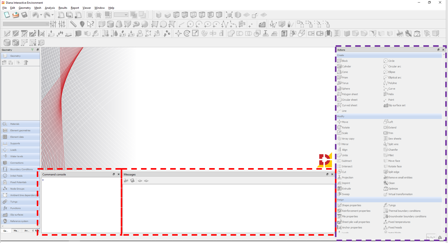
It has been observed that in some cases the legend of the result pictures from Diana is not well adjusted to the picture size. This can be solved by closing/minimising the Command Console and Message box in Diana, before running the script. (But check the Message box after the script is finished to check for warnings/errors!) Besides, it is advised to minimise the Action and Properties boxes, these will be automatically shown when the script is running, hence closing them will not work.
Specific components of the result handling
By default the above function will generate all required result components. The user might want to have a specific result. In this section the sub-functions are explained. These can be used alone, but do require the model to be loaded. You should only run those if certain output needs to be customised, else use the procedure described above.
The convergence graph
The convergence plot is created from the out-file. The graph is generated with the sub-function
viia_convergence_graph():
project.viia_convergence_graph()
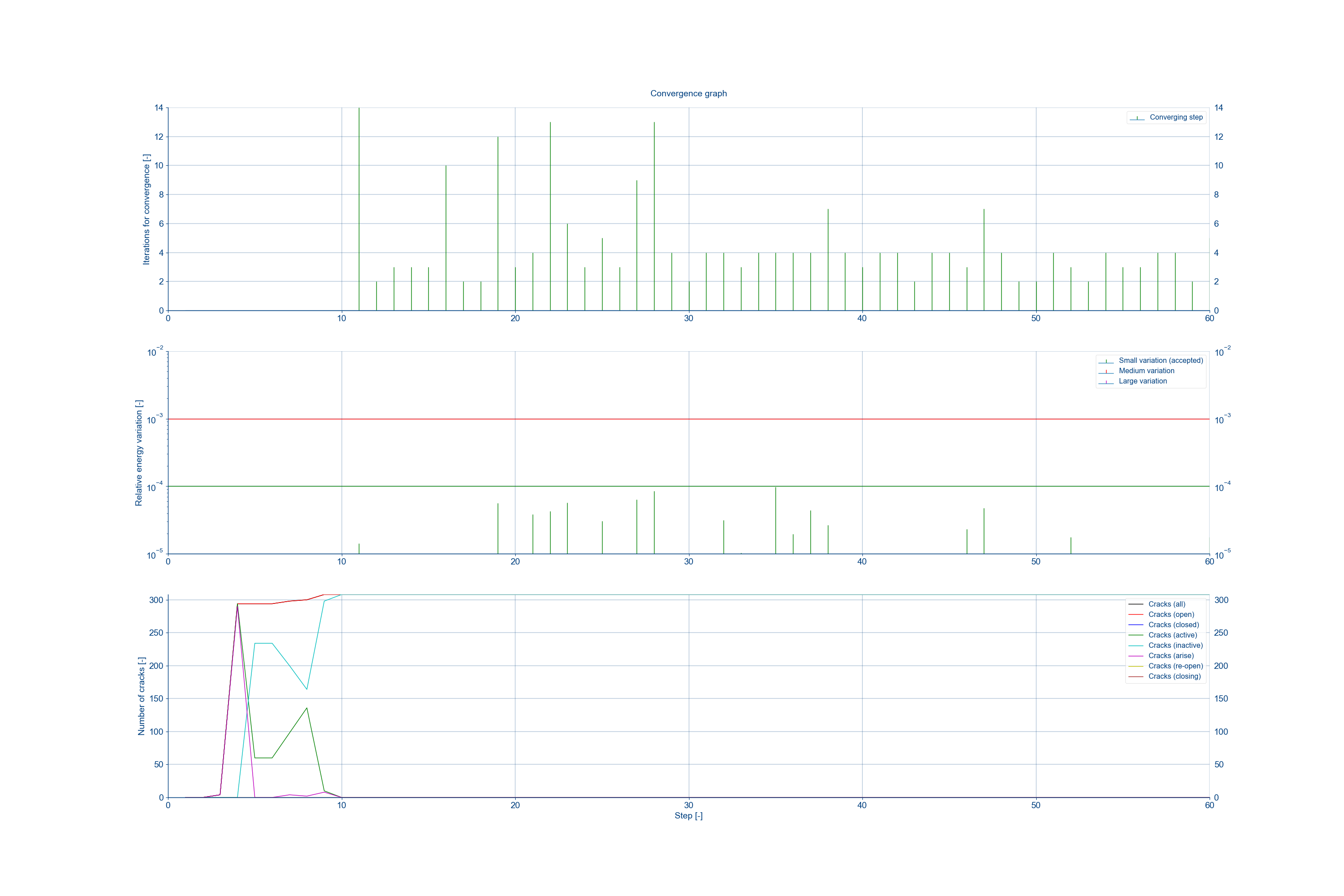
Figure 75 Example of the convergence graph for the analysis.
The base shear graph
The base shear graph is generated right after, based on the OUTPUT 5A and/or 5B result files. The graph is generated
with the sub-function viia_base_shear():
project.viia_base_shear()
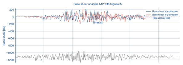
Figure 76 Example of the base shear graph for the analysis.
The out-of-plane displacements plot
Displacements of all the walls are also plotted over the length of the signal, based on the OUTPUT 2 result file. There
are the graphs of the displacements of top, middle and bottom node and graphs showing the relative displacements. The
graphs are generated with the sub-function
viia_wall_displacements() in a subfolder
‘OOP_IP_displacements’:
project.viia_wall_displacements()
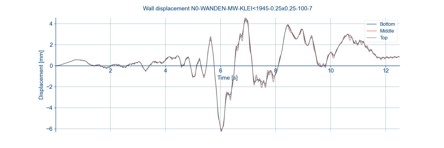
Figure 77 Example of the wall displacement graph for the analysis.
Acceleration graphs
Acceleration graphs are also plotted over the length of the signal based on the OUTPUT 3 result file. The graphs are
generated with the sub-function
viia_acceleration_graphs() in a subfolder
‘Acceleration Graphs’:
project.viia_acceleration_graphs()
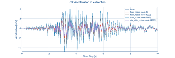
Figure 78 Example of the acceleration graph for the analysis.
Generation of the result pictures
The last part of result generation is the actual result pictures from DIANA. To get those pictures you must run the
resultscript in DIANA. The pictures are generated with the sub-function
viia_create_result_pictures_nlth()
viia_create_result_pictures_nlth(project=project)
The A12 analysis folder should now contain the following images, if applicable:
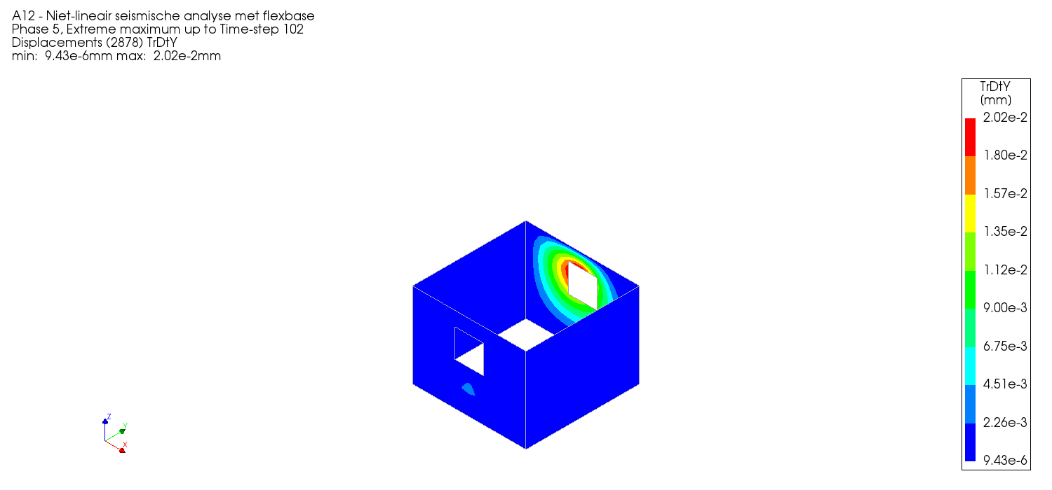
Figure 79 Relative displacements of the walls per storey.
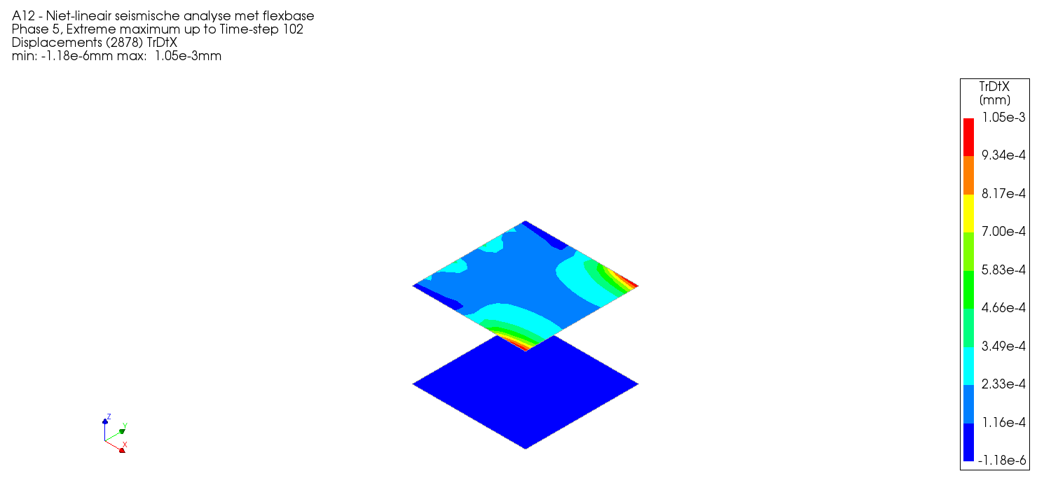
Figure 80 Relative displacements of the floors per storey.
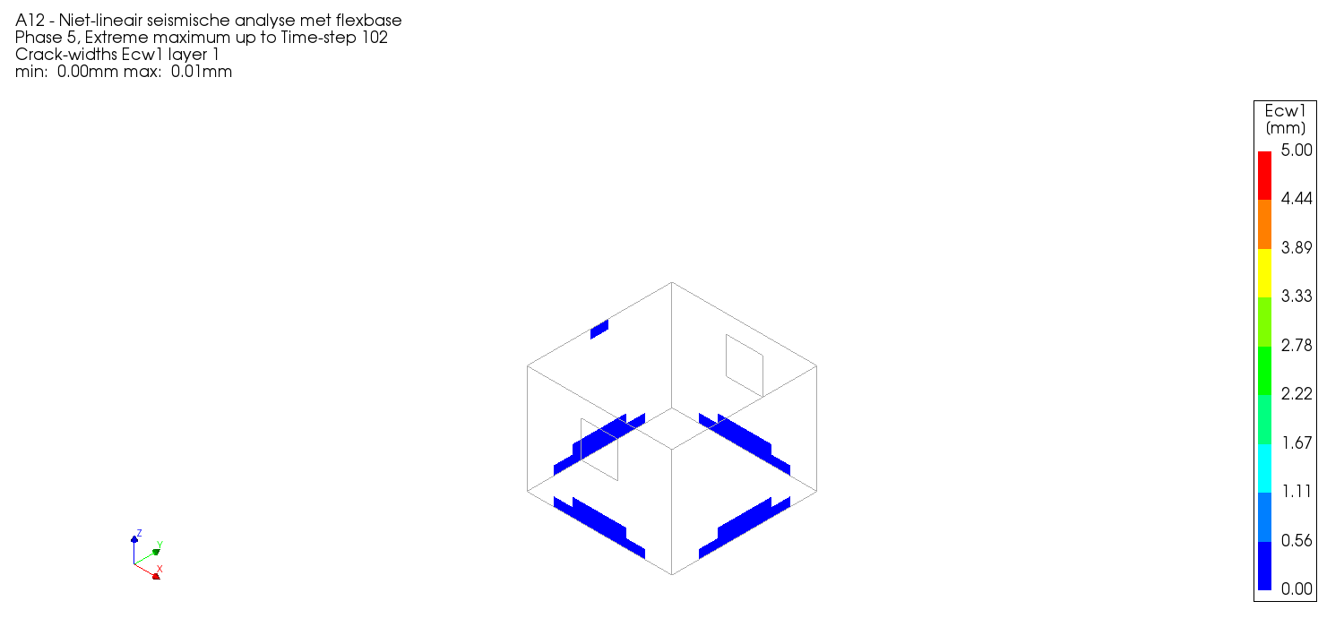
Figure 81 Crack width of the walls per storey in the 1st, 4th and 7th element layers.
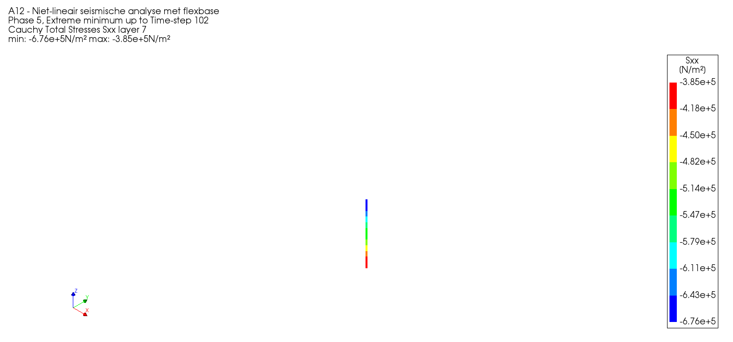
Figure 82 Axial stresses in beams and columns per storey, per material.
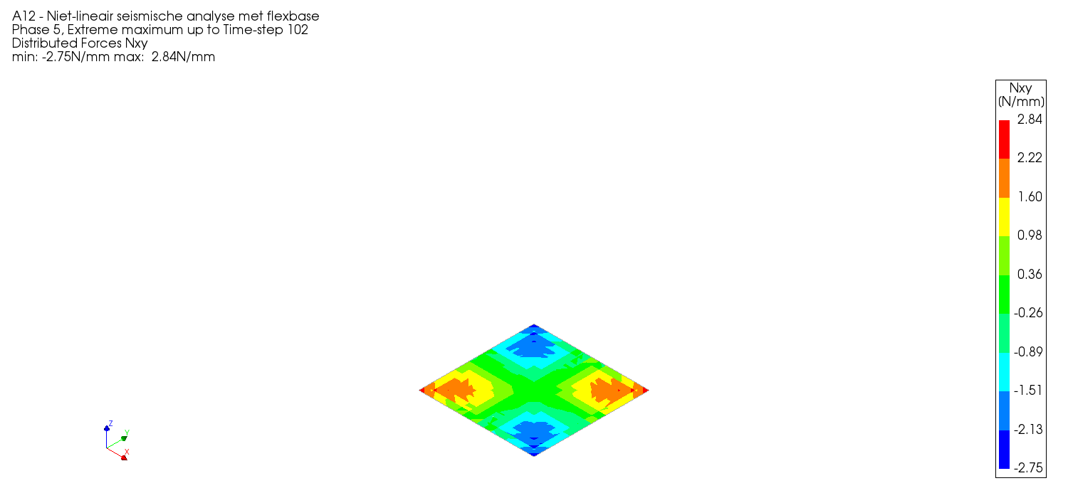
Figure 83 Shear stresses (and, if applicable, strains) in floors per storey, per material.
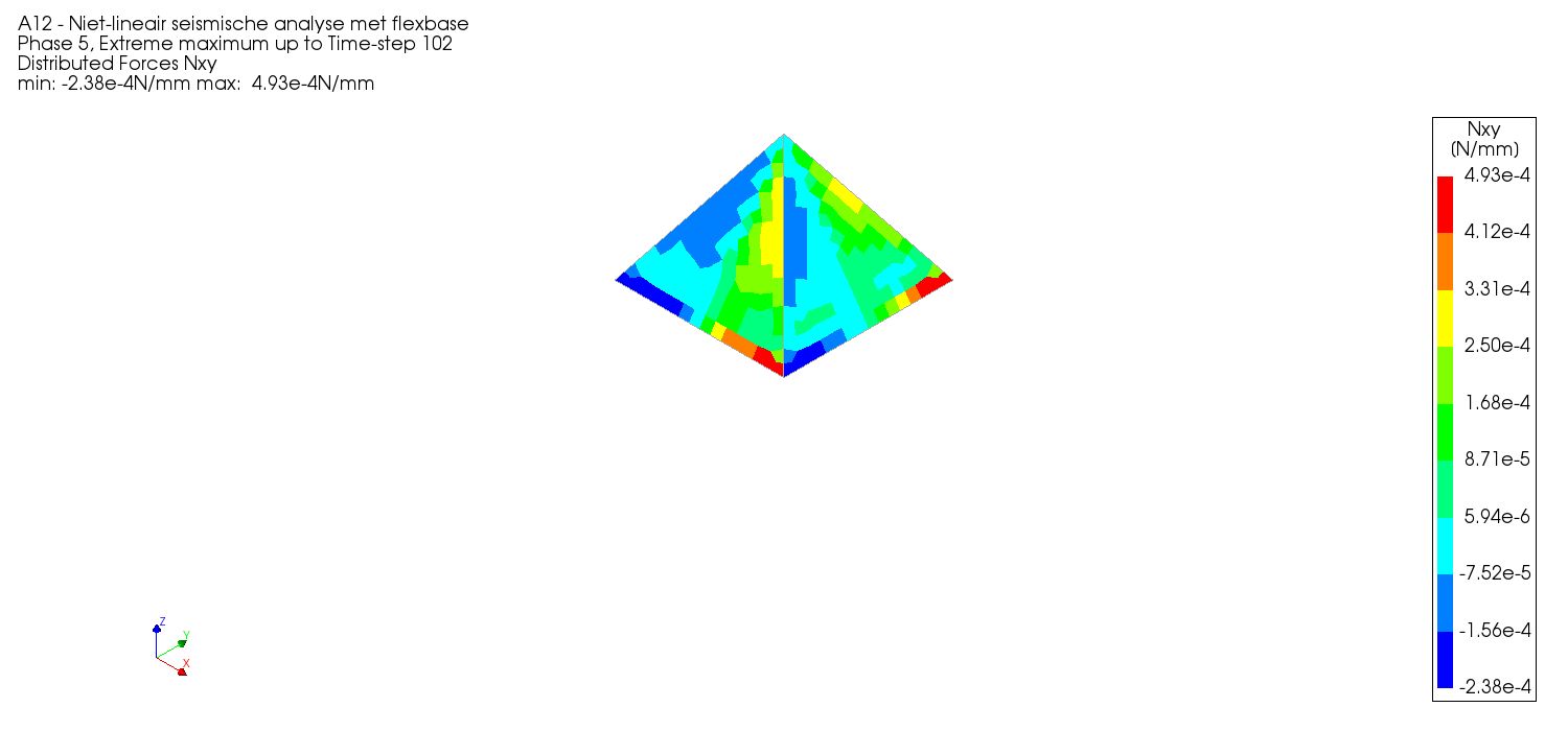
Figure 84 Shear stresses in the roof, per story, per material.
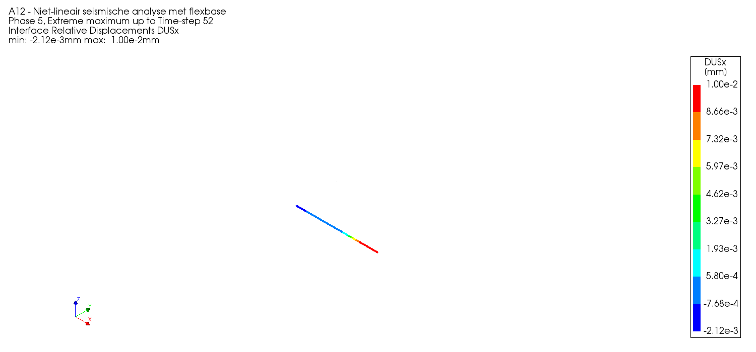
Figure 85 Interface displacements per storey.
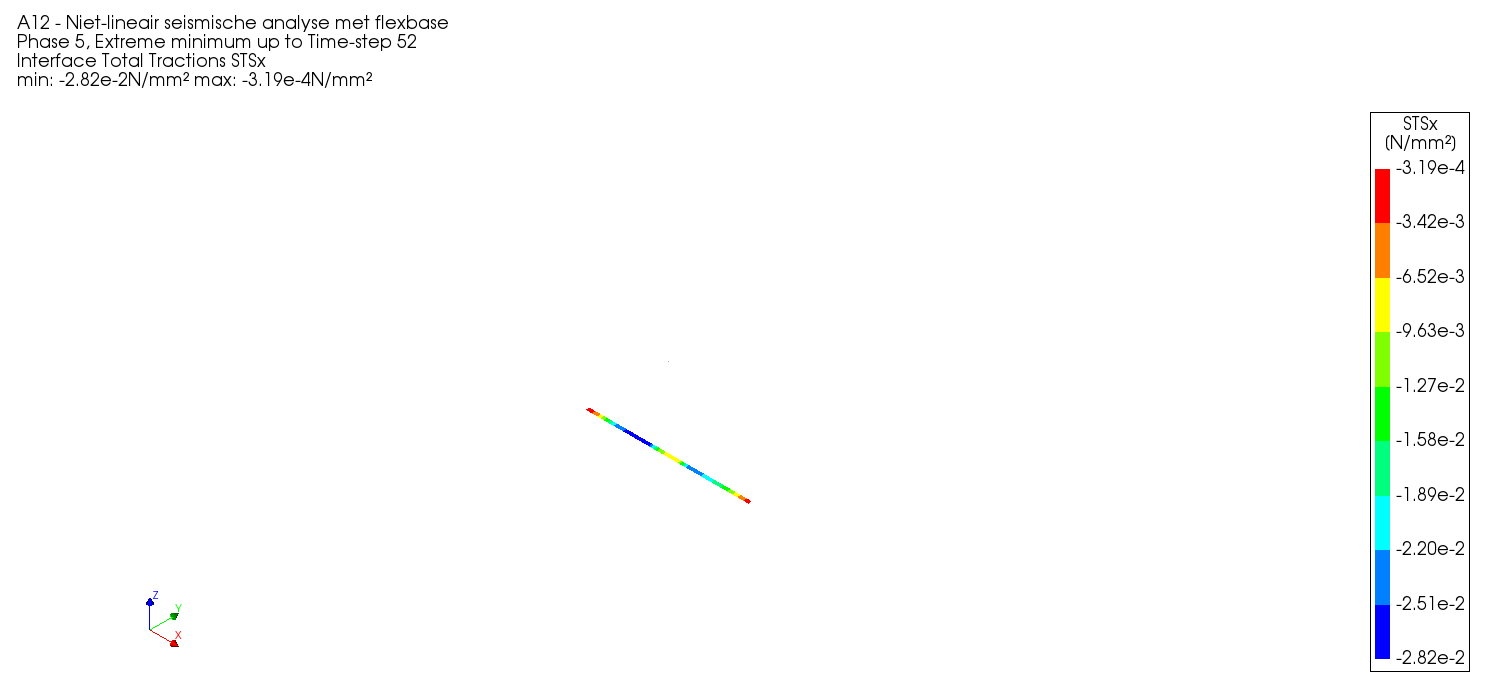
Figure 86 Interface tractions per storey.