3. Phase 2 - Fixed base model phase
The purpose of the analysis model is to give a accurate representation of the mass, stiffness, deformation, force distribution and damping of a building system. This is done by a simplified model (simplified compared to an architectural model). For example small corners or recesses should be neglected, and structural schematisation should be set-up as unambiguous. With this improved model, the numerical process is more stable and the calculations are faster.
In the seismic analyses within VIIA, the fixed base condition is always initially addressed, since this is a less complex model boundary condition that can provide useful insights in the expected seismic performance and it is recommended to be always performed before the flexbase condition. The fixed base is therefore also part of the model check.
The previous phase delivered the model as a json-file. This file is loaded in the mainscript and the boundary conditions, the seismic loads and other settings for the specific analysis are added to the script.
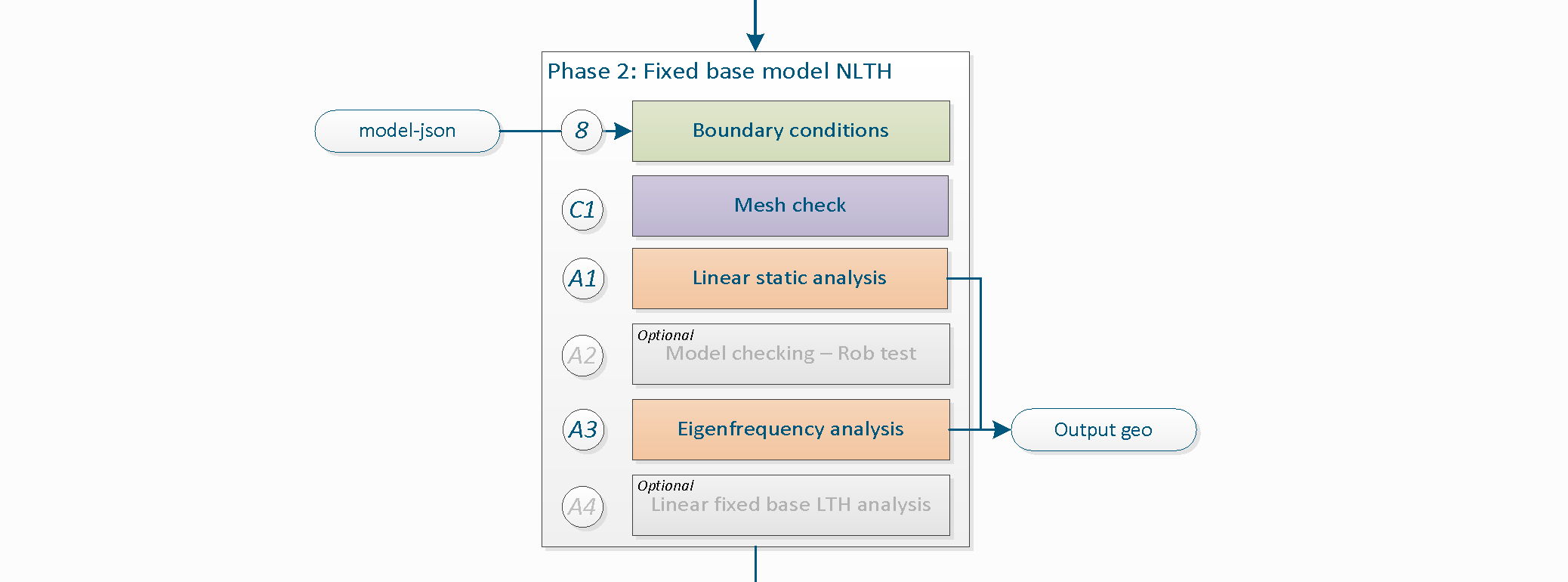
Figure 3.1 Phase 2 - Fixed base model.
Adding complexity to the model should be done in small steps, reducing the time spent on errors, because it is easier to pinpoint the location of the error. With this workflow, time is minimised and quality is guaranteed.
For the NLTH the final assessment is based on a flexbase analysis. In that phase it is necessary to use spring values according to the soil conditions, as observed for phase 3. The steps to run fixed base analysis is to verify the model and stepwise increase complexity.
Note
For each phase various steps need to be performed. The number assigned at the left side of the step description is used to identify the step and to link it with the corresponding item in the python-script. It is not necessary to perform the steps in the presented order. However all steps in a certain phase should be completely finished before moving forward to the next phase.
When the model is finished in the previous phase, a json-file is created containing all information on the model, the properties and the non-seismic loads. The modelscript is now finished and the analyses that are performed on the model are set in the mainscript. The first step in this mainscript is to load the previously created model and set the settings for the analysis. These settings aim at the boundary supports, the loads, the analysis and in some cases the result handling.
The mainscript should already be prepared and prefilled when the installation procedure was performed. Else you can download the template or retrieve it from the viiaPackage. The mainscript is specific for the analysis method. In contrast with the modelscript which is general applicable.
The mainscript is started with the following code:
from viiapackage import *
This loads all functionality required for VIIA. It is not necessary to separately import the haskoning_structural
package. Start the project with viia_create_project() and use the VIIA object number.
The version must be 1 for the existing building assessment. When strengthening measures are applied later in phase 5 the
version is going up.
project = viia_create_project(project_name='811V', version_nr=1)
In case of object parts (separate analyses of building parts as agreed with the client) you need to provide the object part that is involved in the analysis. You can find the object part names on the MYVIIA webtool.
project = viia_create_project(project_name='587M', object_part='Woonhuis', version_nr=1)
The model created in the modelscript in phase 1 should now be loaded. To perform this action the function
viia_read_dump() is available. This requires the json-file as input, for example:
project.viia_read_dump('model/811V-model')
Note that in the mainscript template some booleans are indicated at the top of the script. These have been added for convenience, based on earlier experiences of structural engineers. These can be used to easily switch on or off certain functionality that is explained in the following sections.
3.1. Step 7: Apply the boundary conditions and base motions for fixed base to the model
Different supports are applied in various phases. In this phase (the initial analyses phase) for the simplified model, supports have to be considered as ‘fixed base’. The model can consist of shallow foundations, pile foundation or a mixed foundation. Separate procedures are available for the different types of supports. In case of the mixed foundation both have to be performed.
3.1.1. Shallow foundations
The function viia_create_supports() is available to create shallow foundations in
the model. When the fixed base is applied, the degrees of freedom of the supports are restrained in x-, y- and
z-translational directions and the x- and y-rotational directions.
project.viia_create_supports()
In the example figure underneath the fixed base support has been applied to the model. Note that the check in DIANA should be done when model is meshed, because in Geometry view this can’t be checked properly. The figure shows how the supports look like in DIANA.
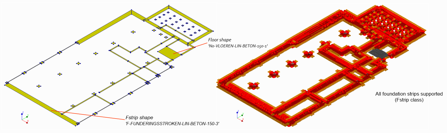
Figure 3.2 Applying fixed base supports for shallow foundation.
The viia_create_supports() function applies supports on all the foundation strip
surface shapes. If it is required to exclude certain foundation strips (when for example piles are supporting that
foundation beam, see mixed foundation), these can be provided to the function in a list:
project.viia_create_supports('FixedBase', excluded_supported_surfaces=['F-FUNDERINGSSTROKEN-LIN-BETON-150-3'])
When additional surfaces are required to be supported (floor on grade) these can be added tin the same function:
project.viia_create_supports('FixedBase', additional_supported_shapes=['N0-VLOEREN-LIN-BETON-150-1'])
These two inputs are shown in the following example:
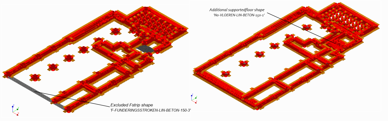
Figure 3.3 Left: Example of excluding a foundation strip. Right: Example of adding an additional supported floor.
When the shallow foundation is created all the supported surfaces can be retrieved from the project. You can use the
viia_create_plots() function to generate a top-view picture of the model with the
supported surface shapes. You can use this function in PyCharm.
project.viia_create_plots(collections=project.viia_supported_surfaces, viewpoint=[90, 0])
3.1.2. Pile foundations
In the fixed base model the pile foundation is created with boundary springs with a relatively high stiffness
(comparable to the MRS approach). Once the A1 static analysis is performed the pile loads are used in the separate
workflow for piles. The function viia_create_piles() is available for creating the
piles in the fixed base model. This function is used as follows (example with one pile only):
pile_coord = [[1.0, 0.3]]
project.viia_create_piles(
    coordinates=pile_coordinates_A, support_type='FixedBase', pile_group='A', cross_section='D200')
It is also possible to start the pile workflow already and get the pile dimensions from MYVIIA. In the following example the piles in group A are already present:
pile_coord = [[1.0, 0.3]]
project.viia_create_piles(coordinates=pile_coord, support_type='FixedBase', pile_group='A')
Here, first the x and y coordinates of the piles are specified. The function will check if there is a foundation beam (modelled as fstrip) present. The function then creates a column with 0.1m length connecting to the foundation strip. The cross section properties are required for the function and are obtained from MYVIIA.
In case of multiple pile groups, the piles should be created per pile group. Specify that the other piles should not be removed.
project.viia_create_piles(coordinates=[[3.0, 0.2]], pile_group='B', new_pile_foundation=False)
If the piles are not (yet) created on MYVIIA it is also possible to provide the dimensions for the piles. These can be specified in two ways:
project.viia_create_piles(
    coordinates=[[6.0, 0.2]], cross_section='D300', pile_group='C', new_pile_foundation=False)
project.viia_create_piles(
    coordinates=[[9.0, 0.2]], pile_shape='square', pile_dimension=0.4, pile_group='D', new_pile_foundation=False)
Note
If no piles are present in your model, remove the template code in the mainscript.
3.1.3. Mixed foundations
Both the procedures for shallow foundation and pile foundations should be followed. The shapes in Fstrip class (the foundation beams and foundation strips) should be excluded from the shallow foundation function when they are located on top of the piles.
3.1.4. Beam rotations along the axis of the beam
When line-shapes are connected to shell elements (used for surface shapes) the rotational degree of freedom of the line shape is not connected to the shell element as that element does not support that degree of freedom. This is fixed by providing line shapes with an auto created boundary condition, that applies a spring value with low stiffness to one of the ends of the line shape.
3.1.5. Base motions
Now the boundary conditions are applied, the base motions can be applied. To perform a dynamic analysis, an acceleration
signal is applied on the supports of the model. The signals are provided via the NEN webtool and are site specific.
MYVIIA already contains the required data. The base motions in three directions are created with the function
viia_create_loads():
project.viia_create_loads('Base motion')
Loads and load-cases are generated with the names ‘Base motion X’, ‘Base motion Y’ and ‘Base motion Z’. The next step is
to apply the base motion signals to these acceleration loads with
viia_add_basemotion_signals():
project.viia_add_basemotion_signals(signal_list=['S1', 'S2', 'S3', 'S5', 'S6', 'S7', 'S9'])
You can select the signals that you want to apply in your analysis. In the final assessment minimum of 7 signals should have been selected. The list shown is the preferred list as the other signals have deviating time-steps. The used importance factor is derived from the consequence class that is defined on the MYVIIA webtool.
It has been agreed with the client to use updated z-signals for which matching has been performed on another frequency domain. Refer to note VIIA_QE_R376_N061, VIIA_QE_R376_N066 or VIIA_QE_R376_N067 for the derivation of the updated matched signals. You can select to use the original signals with the input argument ‘use_unmatched_signals=True’.
3.1.6. Load combinations
After creating the load cases, these must be combined. DIANA only performs calculations from load combinations. In
ABAQUS loads that are defined in a step can be used directly. For a static analysis, a load combination ‘Dead load’ is
created with the function viia_create_load_combination_static(). The function
viia_create_load_combination_rob_test() creates the load combination ‘Rob-test’ that can
be used for the Rob test in step A2. It can also be removed with the function
viia_remove_load_combination_rob_test(). Functions overview in this section are review
in Table 4. To create the load-combination for the seismic analysis use the function
viia_create_load_combination_base_motion() and provide the signal number that needs to
be analysed. The signals should be available (see the loads section on base motions).
project.viia_create_load_combination_base_motion('S3')
3.1.7. Linear material properties
In the fixed base model the material properties should be applied as linear materials. Because in the model script the
materials are created non-linear, for this analyses phase you want to ‘temporarily’ remove the nonlinear material
properties, the functions viia_linear_properties() and
viia_non_linear_properties() can be used. They act as a toggle, to switch on and
off the nonlinear material properties.
3.2. Step C1: Mesh check
After assigning material and completing the building geometry, the model is meshed. Before the model is ready to perform structural analyses, it is important to first go through checks related to the modelling process. This reduces the risk to face issues related to the model in later stages.
Some tools have been developed to assist in the mesh-check. The viia_check_mesh()
function will generate a report that offers insights into the mesh setup. It displays the count of mesh nodes and
elements and a list of the element-types used. Alongside general information, the report includes graphs depicting
distributions.
project.viia_check_mesh()
The function checks for the following aspects of the surface mesh-elements:
Check if the angles of the mesh-element are larger than the minimum angle requirement (VIIA default 15 degrees).
Check if the angles of the mesh-element are smaller than the maximum angle requirement (VIIA default 165 degrees).
Check if the skewness of the mesh-element is smaller than the maximum skewness requirement (VIIA default 45 degrees).
Check if the aspect-ratio of the mesh-element is smaller than the maximum aspect-ratio requirement (VIIA default is 5).
When there are elements present that do not comply to the VIIA requirements, a warning is raised. Review the failing mesh-elements, the mesh should be improved here. In most cases the geometry can be simplified in these locations, else specified mesh-seeding could help to improve the mesh quality. Discuss with your Lead Engineer how to proceed.
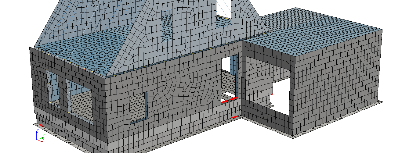
Figure 3.4 Visualisation in DIANA software with the locations of non-complying mesh-elements.
For convenience the DIANA command is printed / logged to visualise these elements in DIANA software. Simply copy paste the line into the DIANA console. The elements exceeding any of the requirements are selected. This syntax is also added at the end of the mesh check pdf report.
You can find more information on this topic in the documentation of the mesh checks in the fem-client.
3.3. Step A1: Linear static analysis
The linear static analysis aims to evaluate the existing condition of the building without applying seismic load (so mostly vertical loads due to self-weight and part of the imposed loads).
After the A1 analysis, the structural engineer should provide the geotechnical advisor the following information if the geotechnical assessment is required:
Mass of the building (including also the weight of the outer leaf).
Surface area of the foundation strip (in case of shallow foundation).
Number of piles in the foundation (in case of pile foundation).
Lay-out of the foundation.
In this way the geotechnical will be able to provide the value of the spring stiffnesses required in Step 9 of Phase 3: Foundation and SSI.
Note
The evaluated structure is an existing structure, so structural elements should not be failing. When in the linear analysis it is found that an element or elements are failing by large margins, it may be an indication of:
Missing important structural elements in the model (maybe considered as non-structural and were taken out from the analysis).
Inappropriate material properties applied to the element.
Elements are not well connected (connections can be either at the edges (e.g.: top and bottom of the element) or also connected through in a contact area (like timber beams fix to timber plates at the roof or timber elements fix to masonry).
By means of the function viia_analysis() a linear static calculation is created and
performed. The following is an example for A1 analysis:
project.viia_analysis(analysis_nr='A1', run=True)
3.3.1. Issues
If problems arise from the results of the linear static analysis, observe the following.
When an analysis converges:
Add result item for stresses to the analysis and analyse again to see where peak stresses occur.
For other possibilities regarding bug fixes see section Convergence
Analysis diverges:
If divergence occurs see section Divergence.
For a better understanding of the dcf-file, read the how-to guide: How to DCF settings.
3.3.2. Results
The result handling is performed automatically when the analysis is created and directly ran in DIANA with the function
viia_results().
The center of mass and weight of the building are logged and together with the area of the shallow foundation sent to MYVIIA, from which the geotechnical advisor will calculate the properties for the flexbase (if geotechnical assessment is performed). The uploaded values can be checked in MYVIIA webtool.
The following results should be observed/checked for the linear static analysis:
3.3.3. Geo-output
When geotechnical assessment is required, the weight of the building is calculated in this analysis and is sent to the geotechnical advisor. Also the area of the shallow foundation is collected. This is automated via the MYVIIA webtool. You can verify if the correct values are sent in model check.
3.3.4. Pile workflow
After the A1 analysis with piles in the model the separate workflow for piles should be performed. This workflow is required to get the properties for the piles in the flexbase model. The workflow is described in ‘pile workflow’.
3.3.5. Reporting
The results of this analysis do not have to be reported. The analysis results are checked during the model check.
3.4. Step A3: Eigenfrequency analysis (optional)
Note
The eigenfrequency analysis in NLTH is only required for models with pile foundations for which the geotechnical assessment is executed.
If you need to execute the eigenfrequency analysis refer to Step A7: Flexbase eigenfrequency analysis for the description of the analysis. The two main differences from the A7 Eigenfrequency analysis are the modified boundary condition at the foundation level and the boundary interface representing the foundation-soil interaction.
After completing all the steps of the fixed base model phase you can continue working on the ‘Flexbase model phase’.