Seismic analysis with NLPO in VIIA
This page contains the protocol for NLPO analyses. It extends on the NLTH part of the protocol.
Warning
This document is not updated for new developments as the NLPO is currently not in the VIIA workflow.
Non-Linear analysis methods and knowledge development
What is NLPO?
In a Non-linear Pushover analysis “NLPO”, incremental static lateral load-steps are applied to the structure (usually at floor level) to determine the yielding strength capacity and observe the post yielding behavior (failure process) of the structure. This is express in terms of the so-called pushover curve (force vs displacement relation). This pushover curve is compared afterward with the spectral seismic demand, provided by the local norm, to evaluate the seismic adequacy of the structure to the required limit state. This conceptualization of the building provides also a straightforward method to not only understand the global actual behavior but also to evaluate conceptually effect of retrofitting scenarios (Figure 196).
The NLPO is a common procedure to assess the in-plane seismic behavior of buildings without or limited horizontal and vertical irregularities since to express the structure into a global unique pushover curve requires certain conditions.
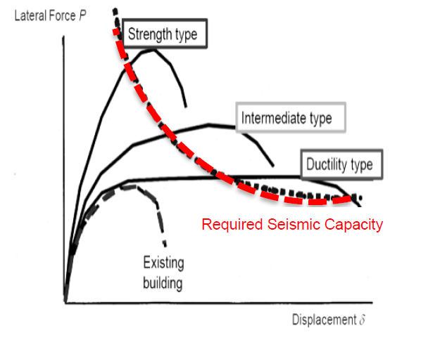
Figure 196 Force vs Displacement.
In NLPO analysis, it is important to have a clear understanding of the probable inelastic behavior and building response depending on both lateral forces and deformation (C2.8.1 NZ 2017). Detailed 3D nonlinear FEM URM models can include aspects that can be addressed directly in the pushover analysis such as torsion, flange effect in laterally connected walls, connections types in between the floors and the walls, variation of the foundation flexibility constrains and influence of the openings in diaphragms. All these considerations are of importance to identify the most probable failure mechanism in the structure.
Figure 197 shows the typical steps in NLPO analysis. For a better understanding of the NLPO process in the context of this protocol, steps are color labeled in light blue for those related to the structural PO analysis (DIANA-FEA software), and in yellow the ones related to the SDOF simplification and determination of the performance point ‘PP’. At the PP, the response of each individual component can be observed back into the structural model.
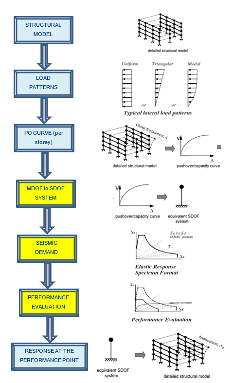
Figure 197 NLPO assessment procedure overview. In light blue steps related to the structural model in DIANA, in yellow the conceptual steps to analyse the SDOF and the determination of the global performance point in the NLPO method.
For the adequate modelling of the structure, the NLPO method requires clear understanding of aspects such as the load flow paths in the structure, condition of connection and identification of seismic primary and secondary structural element. The most important aspects to inspect/identify, with focus in URM, for the NLPO are:
geometry & continuity of primary/secondary structural elements,
recognition of structural and non-structural elements,
connection in between wall-wall and wall-floor,
materials types of the structural elements, and
spanning directions of floors and roofs.
When to use the NLPO method
Low-rise structurally regular buildings with rigid floors are the typical structural type analyzed with the NLPO method in the context of this protocol. Engineering judgment is required to determine the applicability of NLPO in case of complex low-rise and regular mid-rise structures. In case of the NLPO classical procedure, in NPR 9998:2018 it is mentioned that the method is not suitable to be used by itself for large-complex structures and should therefore be complemented if considered necessary with other analyses that would allow to investigate load redistribution and complex inelastic displacement profiles. If NLPO is not applicable, NLTH or MRS-analyses type should be used for the assessment (G.1 NPR).
Diaphragm characteristics are key to determine the feasibility to analyze a structure by means of the proposed 3D FEM model in this protocol. This decision-making process can be observed in Figure 198. For URM structures with flexible (or partly no diaphragm) or an ineffective diaphragm (according to deformation information from the diaphragms check), individual lateral bracing elements (walls) can be assessed independently for both in-plane (IP) and out-of-plane (OOP) actions (NPR G.2 Note 5) and SLaMA procedure may be used. For structures with rigid floors, 3D models incorporated directly torsional effects, but a torsion check is required anyways during the process due to limitations for the maximum allowable eccentricity.
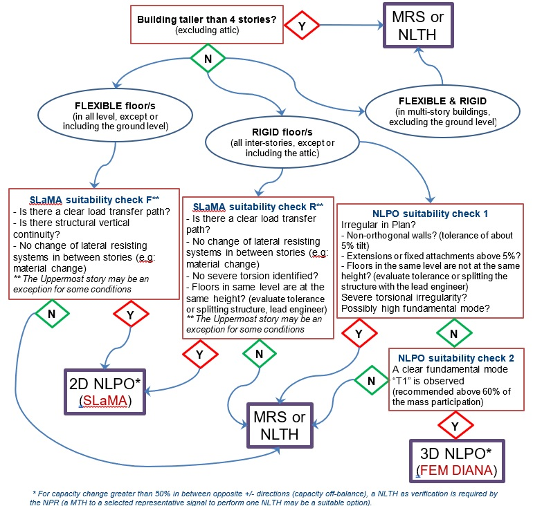
Figure 198 Are the 3D NLPO or 2D NLPO methods suitable for my object? The second NLPO suitability check requires already the 3D object model (part of the structures that are not fixated or considered not fixated by the engineer can be either analysed separately or not assessed if they are not usual living area (NPR 4.3.6.1 note 6)).
The applicability of the NLPO process for a feasible 3D NLPOA is limited to various structural condition that can be recognized previous to start the assessment process by pre-identifying or checking certain building typology characteristics. The aspects relevant to assess the feasibility of NLPO according to the method limitations are overviewed in Figure 198. The criteria included in Figure 198 mention the following aspects of importance for the NLPO method:
Maximum height: NLPO in NPR limited to a maximum of 4 stories (including attics)
Vertical Irregularity: Structural material change in height (high modes influence)
Vertical Irregularity: Strong stiffness change, structural system changes or discontinuity of main structural elements (4.2.3.3)
Higher Modes and Mass Participation Checks: T1 participation factor recommended be greater than 60% for each analysis direction. T1 value limited to 0.9 seconds (G.4.8)
Torsion limitation: The eccentricity should be limited to a maximum 0.4b, where b is the minimum dimension of the building. (severe torsion)
Structure geometry: Initially limitation for a maximum ratio of 4 to 1. (4.2.3.2) in plane, and vertical shape limitations according to 4.2.3.3.
Diaphragms openings: Maximum percentage allowed of openings (10%, to be check)
Diaphragms regularity: All floors in a level should be at the same height (evaluate small height level change tolerance or splitting of the structure together with the lead engineer)
The estimation of the building typology at the beginning of the process NLPO can be useful for the planning of the project leader and for the HC (Head Engineer), since from there the engineer can inferred the type of NLPO analysis to be performed and the expected duration of the structural engineering process. Therefore, it is necessary to inform the project leader regarding the typology of NLPO decided to perform the analysis in order to make a proper initial decision of what method should be followed. Figure 198 schema also suggests other analysis methods when the NLPO method is considered not suitable for the structure.
Phase 1 - Starting phase
Step A0: Simplified NLKA analysis
Note
Only valid for NPR9998:2018.
The here is to use a simplification of the NLKA assessment method presented in the NPR:9998-2018 annex H as an initial conservative way to address walls. It has been observed that walls commonly pass the OOP NLKA check for typical URM house configurations in practice. So, simplification of the procedure is desired, not only to accelerate the process but also to avoid erroneous evaluations. The simplified analysis results are independent of the analysis method, hence valid for NLPO, NLTH or MRS. Nevertheless, in the NLTH and MRS process the out of plane assessment is evaluated currently directly from the structural model.
In the proposed procedure mostly the height of the walls and the location of the walls is of relevance. According to these properties normalized graphs can be created for typical un-reinforced masonry situations. This is presented for example in the image below. Details related to the simplified NLKA can be found in the following link: (Simplified NLKA)
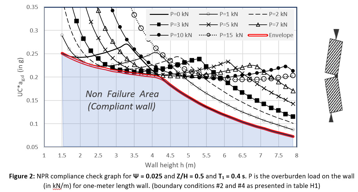
Figure 199 Non failure area in the simplified NLKA assessment according to the VIIA report XXXX (UC + unity check).
Phase 3 - Flexbase model phase
For NLPO the additional displacement capacity attained from the equation G.16 presented in section 8 of annex G of the NPR9998 is usually very small. It may be neglected by the structural engineer in analysis A11.
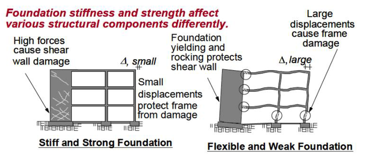
Figure 200 Stiff and Strong foundation vs. Flexible and Weak foundation.
When you create a shallow foundation and/or piles in your model, after creating the fixed base foundation. The fixed base shapes will be removed first.
Step A5: MRS analysis of floors / roofs
Note
A5 type analysis is not supported in ABAQUS.
To check the roof and the floors, an MRS analysis in DIANA can be performed. The MRS should be performed with a fixed base or a flex base with stiff values. To perform an MRS analysis the following steps should be taken:
Perform eigenfrequency analysis first based on fixed or flexbase model (see Step A3: Eigenfrequency analysis (optional) or Step A7: Flexbase eigenfrequency analysis)
Create the analysis according to the procedure in the how-to guide: How to MRS analysis
Show in results the ‘superposition type CQC’ and look into the values of NxyH and NxyL for plates. And SeqH and SeqL for beams. These values should be compared with the values in the UPR chapter 9.
Analysis
By means of the following function, the modal response spectrum analysis can be applied to the structure. The preferred
setting for the run argument of viia_analysis() is ‘True’, indicating direct
calculation in DIANA when running mainscript in DIANA. Initially set the number of eigenmodes to 10. The number of
modes should be determined in the A3 or A7 analysis and consider at least 70% of the participating mass.
project.viia_analysis(analysis_nr='A5', run=True, nmodes=22)
Issues
For a better understanding of the dcf-file, read the how-to guide: How to DCF settings.
Results
Refer to chapter 9 of Basis of Design for NLPO.
Reporting
The results should be reported in HowToReport_AppendixResultsAnalysis-label.
Step C2: Model check
Location of model check files
The files used for the model check and the report that is generated should be saved to the following box-folder:
Objectname > 05 Beoordeling Seismische Capaciteit > 03 Beoordeling Seismische Capaciteit > 03 NLPO > 01 Concept > Model check
Step A11: Nonlinear flexbase push-over analysis
Note
A11 type analysis is not supported in ABAQUS.
In this section, specific details related to the NLPO analysis execution according to the NPR9998:2018 are detailed. A ‘iterative procedure’, as mentioned in Eurocode 8 (EC8), has been used by the NPR: The Capacity Spectrum Method. This concept has been introduced in several guidelines such as the ATC-40 [ATC, 1996] and the NEHRP [FEMA-273, 1997]. In the CSM method, the non-linear pushover curve becomes a capacity spectrum when the curve is transformed into the equivalent acceleration-displacement response spectrum.
Output for the Geotechnical group static and seismic check of foundations is reported after performing this step. For the geotechnical evaluation, it must be addressed the condition at the foundations. Typically, foundations geometries are many times assumed since few information is available and visual inspections difficult to be conducted. If the terrain below the foundation or the foundation itself is failing by large margins, this may be an indication of inappropriate geometry assumption.
Steps in the NLPO Procedure
According to the NPR9998:2018, the nonlinear seismic capacity curve to be used in the NLPO assessment can be generated by:
a simplified hand calculation mechanistic method such as Simplified Lateral Mechanism (SLaMA),
a pseudo-nonlinear analysis using iterative elastic analysis,
an equivalent ‘macro-element’ building frame formulation or
full nonlinear finite element modelling of the building structure taking into account physically the geometrically nonlinear behaviour.
It is expected that for a ‘type d’, a 3D fem-model will present capacities greater that those estimated by other methods. This is recommended to be checked by the NPR and is further commented in stage 4 of the proposed procedure.
The following 10 steps or stages elaborate the NLPO curve and compliance criteria as proposed by the NPR9998:2018. It includes assumptions and special considerations that apply only for low-rise URM structures and the procedure presented here is proposed for capacity curves generated from full non-linear finite elements 3D-models in accordance with G.1.(1) c and G.6.1.(1) d of the NPR. In this procedure, the mean values of the material properties are used (G.4.2.(1)) with the inclusion of a reduction in the material properties (ɣm=1.1) (G.4.5(2)).
Stage 1: Compute the nonlinear pushover capacity
The capacity shall be determined using a (best estimate) approach for material and geometrical properties, based on mean values. An adequate inspection of existing buildings is of importance to attain reliable pushover curves from the model. Inspection requirements for existing buildings are detailed in clause 1.8 of the CVW Guidelines and NPR9998:2018 Appendix A. In case of typical CC1b structures, NLPO assessment can initially be conducted based on structural drawings only, but the evaluation assumptions should be checked in later stages (GSAT guidelines, not recommended for old structures). For CC1b buildings, database information for local soil condition can be used (flowchart CVW Guidelines MOVED TO SHAREPOINT) (to be consulted with the geotechnical department).
The most relevant aspects to inspect to attain quality NLPO assessments are the ones related to the following information:
Geometry and continuity of primary structural elements,
Recognition of structural and non-structural elements,
Connection in between wall-wall and wall-floor (assumption type at the connections), and
Materials and spanning directions of floors and roofs.
When applying the desired incremental PO load, various displacement control points are defined for the structure according to the type of NLPO; a SDOF-system or Subsystem NLPO. The figure presented below shows an example of allocation of control points in the structure for both conditions.
The positioning is in accordance to the flexibility of the walls and floors. For flexible floors, control points should be added to each structural wall direction (assessment line or subsystem as in the figure below). Here, the base shear to be used in the PO-curve is calculated for each line (or sub-system) according to its tributary area. For rigid floor conditions, control points can be assigned in the floor diaphragm (center of mass to include torsion effects) and the total base shear is used for the construction of the PO-curve.
The reported capacity curve, PO curve, is different for building with flexible floors and for building with rigid floors:
For buildings with flexible floors the point should be at the attic level or roof level for flat roofs (point 2480 for line A in ±Y and line 1 in ±X, point 3044 in line B in ±Y and line 2 in ±X) (see the figure below left).
For buildings with rigid floors the reported capacity curve is the one at the attic level or roof level for flat roofs (point 2734 in ±X and ±Y) (see Fthe figure below right).
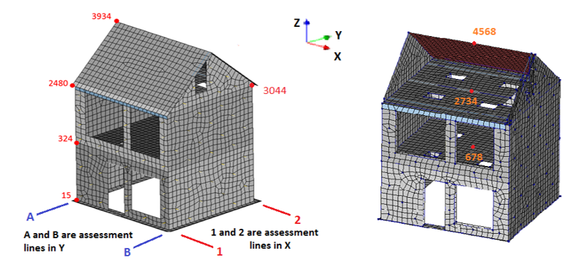
Figure 201 Multi line NLPO assessment (Left) and Single-system NLPO assessment (Right).
For each system or subsystem, a representative PO-curve is selected according to the ‘most critical’ direction and load combination identified for the model. Here, curves should be also provided for both main orthogonal directions (X and Y) and must be tagged as ductile or brittle response since this is of relevance to determine the allowable drift limit. The most critical PO-curve in URM can be identified by inspecting the curves, the crack pattern in the FEM and/or by estimation of failure modes according to the equations in section G.9 of the NPR 2018.
The differences in the definition of the structure presented in the figure above as a whole system or in two subsystems can be observed in the figure underneath. Here one of the main differences noticed is a higher value of elastic stiffness and ductility of the systems. The additional base shear in a system formulation is not an aspect that can be evaluated still in the figure below since the effective mass will be higher for the whole system than to the one of each sub-system.
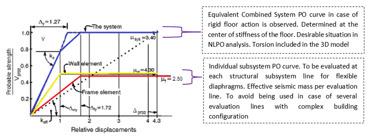
Figure 202 NLPO curves.
Settings to obtain the Push-Over curve:
The Push-Over curve is performed by means of the DIANA software. Once that the model is completed and the Detailing and Non-Linearities have been added to the model, the NLPO curve can be constructed. To speed the set-up process required by DIANA to obtain the Push-Over curve and execute the analysis in a more efficient way, functions have been developed in Python. These functions have different arguments based on the typology of NLPO analysis: SDOF NLPO or Subsystem NLPO assessment. There are functions available for creating the loads and the combinations.
SDOF NLPO
# SDOF NLPO
# Create LOADS

# Modal pushover load pattern
project.viia_create_loads('Push_over_modal', mode=7)

# Uniform pushover load pattern
project.viia_create_loads (Push_over_uniform)
Subsystem NLPO
# Uniform pushover load pattern
project.viia_create_loads ('Push_over_equivalent_acc')

# Triangular pushover load pattern
project.viia_create_loads (Push_over_triangular_load)
To create the load combination the function: viia_create_load_combination_push_over can be used. The functions are containing all the information regarding the settings required to perform the NLPO analysis in DIANA software. An example of the settings contained in these functions are: number of load steps, the load set, the settings connected with the regular arc-length control, the iterative method, the convergence norm settings, the properties of the output, etc.
Note
The DIANA results are considered reliable until the point in which the steps are converging; for this reason, in case of no-convergence or divergence, is mandatory to try to change some settings in the analysis in order to see if the outcome is improving and a better convergence is reached in the model. DIANA SETTINGS:
In DIANA as a first set of parameters the engineer can use:
Iterative Method | Convergence Norm
Maximum number of iterations: 20
Satisfied all specified norms: on
Method: Newton Rapson
Displacement: on (tolerance:0.01, No Convergence: continue)
Type: Regular
Force: on (tolerance:0.01, No Convergence: continue)
First Tangent: Tangential
Line Search: on
Note: check in the DIANA model that these settings are correctly set for the analysis.
In addition to the set of parameters (1) the arc-length control can be added in the load steps of DIANA. In this case a first push-over analysis is performed to see the behavior of the building without the arc-length control. The goal of this first ‘push’ is to determine the final step of the elastic range. From the end of the elastic range onward, the arc-length control is added in an additional executive block in DIANA. In the Arc Length Control setting, nodes need to be selected. In case the building has a sloping roof, the engineer must take the nodes located at the top edge of the roof; if there is a flat roof, the top nodes of the walls, parallel to the push over direction, located at the last story of the building need to be selected.
If, with the previous set (2), an early no-convergence is found, or the results are not good another set of parameters can be used:
Iterative Method
Convergence Norm
Maximum number of iterations: 20
Satisfied all specified norms: on
Method: Secant (Quasi-Newton)
Displacement: on (tolerance:0.01, No Convergence: continue)
Type: BFGS
Force: on (tolerance:0.01, No Convergence: continue)
First Tangent: Previous Iteration
Line Search: on
In addition to the set of parameters (3) the arc-length control can be added in the load steps of DIANA. In this case a first push-over analysis is performed to see the behavior of the building without the arc-length control. The goal of this first ‘push’ is to determine the final step of the elastic range. From the end of the elastic range onward, the arc-length control is added in an additional executive block in DIANA. In the Arc Length Control setting, nodes need to be selected. In case the building has a sloping roof, the engineer must take the nodes located at the top edge of the roof; if there is a flat roof, the top nodes of the walls, parallel to the push over direction, located at the last story of the building need to be selected.
For a more detail explanation about the convergence refers to the section Validation of the obtained Push-Over Results in this document.
The decision of the parameters used are based on the compliance criteria detailed in the basis of design report UPR
( Uitgangspuntenrapport, v1.0: UPR-NLPO). Finally, the
function viia_analysis() performs a non-linear push-over analysis for the structure.
Examples of functions available are:
SDOF NLPO
project.viia_analysis('A11')
Subsystem NLPO
project.viia_create_analysis('NLPO', 'ML', 'X_pos')
Stage 2: Convert the capacity curve into a SDOF-system
The global behavior of the structure can be simplified to an equivalent simple degree of freedom system SDOF-system. This is shown in the figure underneath.
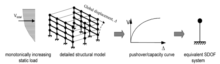
Figure 203 NLPO curves (ref: FEMA 440).
In the conversion to a SDOF-system NLPO formulation, the global structural ductility capacity is generally governed by the dominant inelastic mechanism that contributes most to the plastic deformation of the system. The choice may not be obvious, so it is advised to consult a senior structural engineer. For the case of the Subsystem NLPO formulation of the structure, several SDOF options will need to be evaluated (the case of structures with flexible diaphragms, or a combination of rigid and flexible floors).
A generic deflection profile is shown in the the figure below (a) (C2.5(a) NZ 2017). According to the elastic deflection profile and mass distribution at each floor, the transformation of the generalized nonlinear pushover capacity curve into an equivalent SDOF-system (figure below (b)) is achieved as follows (G.4.2 NPR):
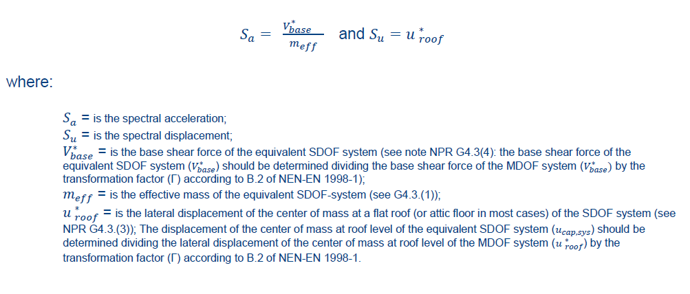
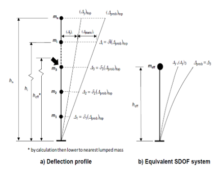
Figure 204 Deflection profile (a) and Equivalent SDOF system (b) (in this picture Δ is equal to Φ)
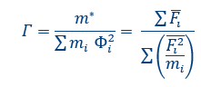
The effective mass m_eff (m* in EC8) is determined by the equation below, where Φ is the normalized fundamental mode of vibration (vector normalized to the displacement of the top level). The mass of an equivalent SDOF system m^* (m_eff) is determined as:

The deflection at the top of the building is taken as 〖〖(Φ〗_prob)〗_top and the deflections at the assumed positions of the lumped masses are taken as δi〖〖(Φ〗_prob)〗_top where δi represents the normalized deflection profile at the level i. Guidance on various deformed shape profiles can also be found in literature ( Priestley et al.,2007;Sullivan and Calvi,2011) ((C2.4 NZ 2017). Other possibility is to use the elastic displacement values from the PO curves per story observed at 60% of maximum base shear (as commented in stage 3). The transformation factor used to estimate the effective height and displacement capacity values (u_(cap,sys)) of the structure is given by the following equation according to the EC 8:
The effective height h_eff of the figure below is determined by dividing the roof height by the transformation factor Γ. The roof height is defined at the attic floor and not the top of the roof (NPR G.4.3.(2)). The spectral displacement capacity ‘u_(cap,sys) (see the figure below) is consequently computed as the displacement of a MDOF divided by Γ. Γ can be assumed equal to 1 in case of structures with a maximum of 2 story’s and one attic height (so an MDOF with 2 concentrated masses) as commented in the NPR9998:2018.
For the case of URM buildings, these typologies usually present essentially systems with their mass distributed over the height, with barely 10-20% of the seismic mass contributed by floors and roof for buildings with timber floors and lightweight roofs (C8.9.4.4 NZ 2017). When estimating the seismic mass (note that seismic mass is different from effective mass!), the mass of the lower half of the bottom story is ignored for the determination of the lumped mass at each level, such as the common practice in concrete building constructions (C8.9.4.4 NZ 2017). This assumption has been adopted and explained in the GSAT-procedure (GSAT Manual V2. 3.2.4) and it can be observed in the figure below.
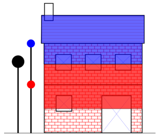
Figure 205 Seismic mass lumped at floor-level (ref: GSAT Volume 2).
Stage 3: Bilinear PO capacity curve for the SDOF system
The bilinear PO curve calculated from the previous step can be linearized for the building system/subsystem using the following procedure:
Calculate the initial stiffness (K_init) at 60% of the maximum base shear capacity;
Find the displacement capacity of the equivalent SDOF-system (‘u_(cap,bilin)) from the PO curve calculated in the previous step. The ‘u_(cap,bilin) is calculated when the capacity of the system drops down to 80% of the maximum base shear of the plateau (view figure below). Additionally, the ‘u_(cap,bilin) value in case of method analysis ‘type d’ should not exceed the inter-story and effective height drift limits as defined in Table 15. In the table, drift limits at the effective height can be evaluated for URM up to 2 story’s. For other URM, RC and Steel structures the inter-story drift limit should directly check at every story in the figure (a) above. This procedure can be done by inspecting the Φ values. The failure mechanisms, in analysis type d, can be determined from crack patterns directly at the FEA; with aid, if necessary, from the equations described in NPR section G.9.
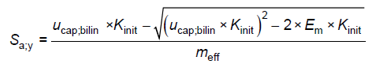
The plateau spectral acceleration capacity ‘S_(a,y) of an equivalent bilinear elasto-plastic PO curve for the system is calculated by the equal energy criterion following the next expression (represented graphically in figure below (a)):
The bilinear formulation is extended up the displacement capacity of the system u_(cap,sys), defined as 50% of the maximum base shear capacity drop. (this can be observed in the figure below (b)). Similarly to ‘u_(cap,bilin), the ‘u_(cap,sys) value should not exceed the inter-story and effective height drift limits as defined in Table 15.
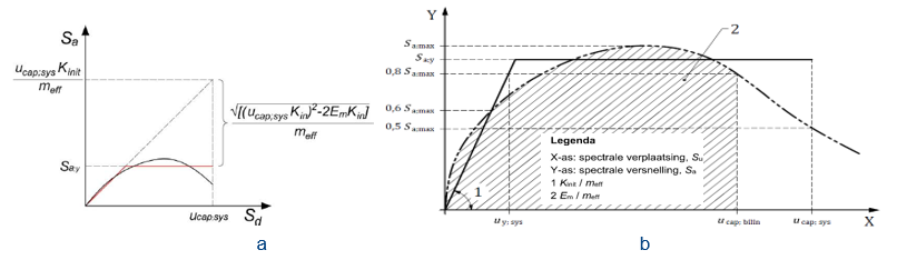
Figure 206 Construction of the bilinear Capacity spectrum parameters. left (a), right (b).
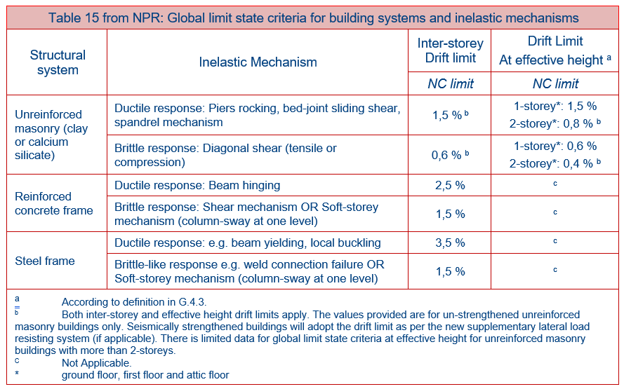
Table - Global limit state criteria for building systems and inelastic mechanisms (from NPR9998:2018).
Stage 4: Minimum PO capacity check according to Note 2 NPR section G.6.1.(4)
Note 2 of the NPR states that for the analysis of “type d”, the finite element model may be checked against a simplified analytical method to ensure that the base shear capacity calculated with the finite element model is not less than the capacity calculated with a simplified analytical method. To fulfil this check, the sum of the resistance capacities of the all lateral resistant elements, overviewed previously to determine brittle or ductile response (example: G.9 section for URM), can be done. The sum of capacities of all elements in a system or subsystem is the theoretical maximum possible lateral capacity that is commonly much lower than the one obtained from 3D FEM models.
For details on the expected failure modes according to the crack patterns and the shear capacity equations consult VIIA report VIIA_QE_R1674_N002 “Validation of masonry material model for NLPO analysis in DIANA FEM software”.
Stage 5: Determination of the global structural ductility of the SDOF, μ_sys
The system ductility, μ_sys, is calculated by the following expression:
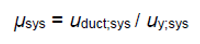
where ‘u_(y,sys) is the yielding ductility(displacement) of the Bilinear PO curve as observed in the figure (b) above, and ‘u_(duct,sys ) is the minimum of either the lateral NC displacement capacity of the equivalent SDOF system (\ ‘u_(cap,sys)) or the intersection of the nonlinear capacity curve and the ADRS seismic demand curve (see G.4.2.(6), called later on ‘u_(int )).
The global structural ductility is governed by the dominant inelastic mechanism that contributes most to the plastic deformation of the system (Note 4 G.4.2). For structural systems with well-distributed and defined plastic hinges of similar ductility capacity, the local structural ductility can be taken as the global ductility capacity.
Stage 6: Equivalent viscous damping ratio, ξsys, and the spectral reduction factor ηξ
The spectral reduction factor is calculated as:
For mixed ductility of inelastic mechanism systems (Subsystem NLPO), a base-shear contribution weighted approach is used to compute the achievable system equivalent viscous damping, ξ_sys, as follows:
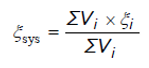
where Vi and ξi are the lateral shear capacity and the viscous damping of each subsystem. Several methods can be used to estimate the system ductility based on the global ductility. A generic formulation is:
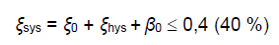
where the system damping is limited to 40% and is described as the sum of the inherent damping ξo (5% for UMR), hysteretic damping ξ_hys and soil damping βo. For the hysteretic damping, the formulations in Table 16 apply.
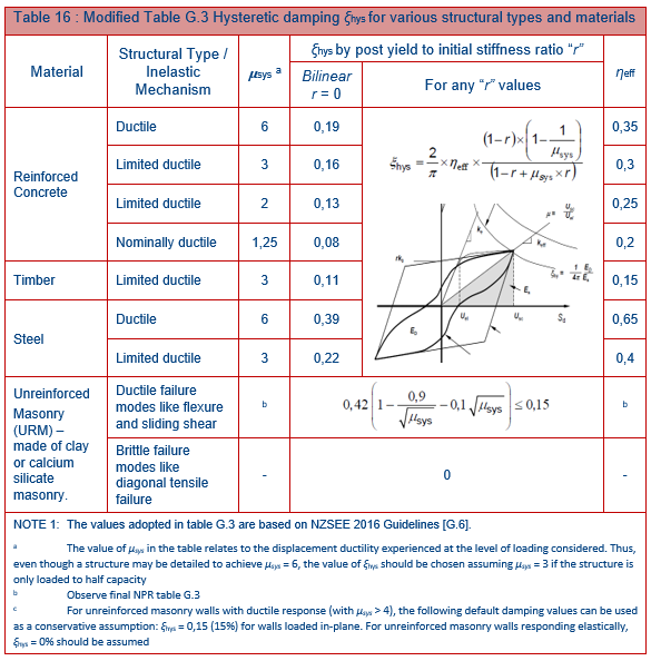
Table - Modified Table G.3 Hysteretic damping ξhys for various structural types and materials.
The effects of the damping radiation (or flexible-base damping ratio) at the soil can be obtained using the following expressions:
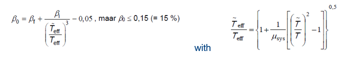
where βo is limited to 15%. With the fundamental periods for the fixed base designated as (T) and for the flexible base designated as (T̃).
An initial ductility value of the system, u_sys, can be estimated from table G.3. For residential buildings up to 2 stories, the soil damping may be neglected (β_0 = 0) (NPR 2018, table G3). β_f is the foundation damping ratio and β_i is the inherent fixed base damping ratio, usually taken to be 0,05.
The following graph in the figure underneath, can be used to estimate β_f for common ground conditions in Groningen (e/rx =0 NPR)
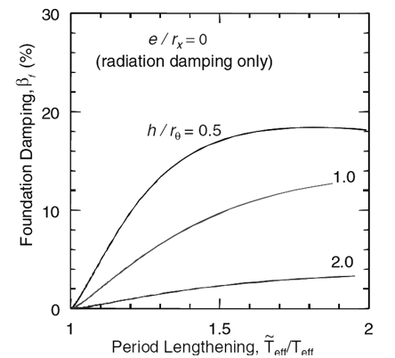
Figure 207 Estimate β_f for common ground conditions in Groningen.
where h in figure is h_eff of the SDOF, and rθ is the foundation radius of rotation calculated as:
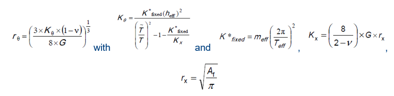
where A_f is the area of the foundation footprint of interconnected foundation components, r_x is the equivalent foundation radius, G is the soil shear modulus, v is the soil Poisson ratio, Kx is the translational stiffness of the foundation, K* fixed is the effective structural stiffness of the SDOF system (calculated by the equation or figure underneath (figure G.5 NPR, where K*fixed= K_eff)), and K_θ is the effective rotational stiffness.
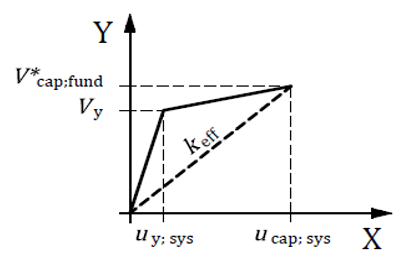
Figure 208 Graphical description of K_eff
Stage 7: Generate the modified inelastic Acceleration-Displacement Response Spectrum (ADRS) demand curve
The inelastic ADRS can be calculated from the elastic ADRS by multiplying by the reduction factor, ηξ defined before. The shape is calculated then according to the following formulation:
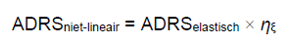
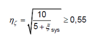
where η_ξ should be greater than 0,55 (this is about a maximum of 20% damping ratio). The result of the previous expression corresponds to the inelastic demand spectrum and can be observed graphically in the figure underneath. The elastic corner frequencies for the ADRS are estimated from the NPR webtool: https://seismischekrachten.nen.nl/map.php
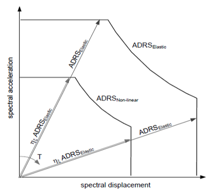
Figure 209 ADRS elastic and ADRS non-linear.
Stage 8: Determine the inelastic seismic demand corresponding to the nonlinear capacity curve
The inelastic seismic demand corresponding to the bi-linearized non-linear capacity curve, S_int (S_int = u_int, (as observed in the figure (a) and (b) below), is the spectral displacement of the modified ADRS demand curve that corresponds to the effective period, T_eff, of the structure (a). T_eff, computed as G.4.3(5), with K_eff is equal to:
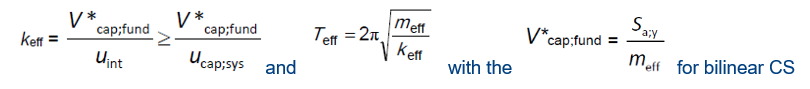
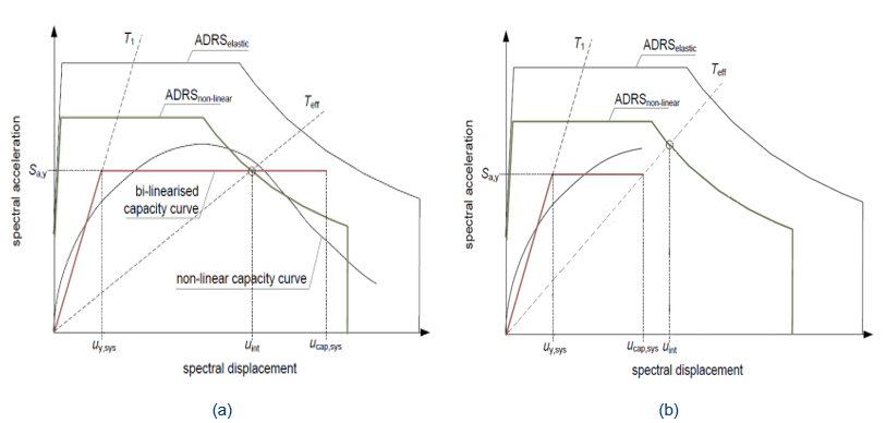
Figure 210 a) T_eff at the intersection in between the spectral capacity and the spectral demand and b) T_eff at the maximum spectral displacement capacity point.
Stage 9: Check of the achievable ductility at the seismic response point
Check whether or not the achievable ductility at the seismic response point (u_int) corresponds to the ductility factor of the system as determined in provision (5) and, if necessary, iterate the provisions (5) up to (8) to find the expected performance point “PP” (where the ductility found at u_int is equal approximately equal to the new calculate u_sys, observe appendix B). For unreinforced masonry walls with ductile response (with 𝜇_𝑠𝑦𝑠 >4), the following default damping values can be used as a conservative assumption: ξ_ℎ𝑦𝑠 = 0,15 (15%) for walls loaded in-plane. Here the iterative process may not be required if the calculated u_int yields in a ductility over 4.
Stage 10: Global capacity-to-demand compliance check
The ratio of the capacity-to-demand points along the secant stiffness (T_eff of the SDOF-system) is useful to assess the global capacity-to-demand compliance check in the NLPO method. The ratio of ‘u_(cap,sys) to S_int (where S_int is equal to last value of u_int attained from the iterative procedure in (9)), referred to as %NBS (in the New Zealand norm), calculated after the (9) is the capacity-to-demand ratio of the system. If the spectral displacement at the T_eff is greater than the ‘u_(cap,sys) value (figure (b) above), the structural capacity is not sufficient (will exceed the near collapse limit state). The maximum value of reference acceleration, ‘a_(g,d), can be found by intercepting the ‘u_(cap,sys) with a reduced intensity inelastic ADRS (at the constant maximum allowed damping value). Values of capacity to the demand ratio %NBS = ‘u_(cap,sys)/S_int lower than 1 are found as Non-Compliant with the NPR. Structures with a %NBS = ‘u_(cap,sys)/S_int higher than 1 are found as Compliant with the NPR 2018.
The %NBS is a parameter that may be used to parametrize how inadequate the structure is. By grouping %NBS values, different risk categories can be defined. The comparison of risk categories for different structural systems is a useful parameter to determine in an efficient manner possible a standardized intervention strategy (see Section 6 Retrofitting).
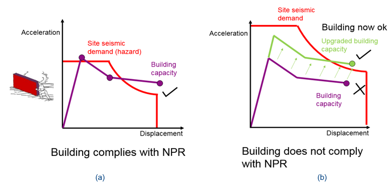
Figure 211 In-Plane capacity of the building compliance check a) Complaint according the to 2018 NPR and b) not-compliant according to the 2018 NPR.
Note
In order to perform all this process a MathCad tool has been created and also different functions are included in the NLPO script to perform this step. The aim of these two tools is to do the NLPO check in a straightforward manner. In the MathCad tool all the steps are noted and aided graphically. The inputs and the corresponding output are highlighted. Here, an example of the report generated by the MathCad tool can be observed.
At the end of this process, the following outputs required to be accounted for each of the following categories:
Foundation check
Report static vertical loads and lateral load for the dominant PO-curves at the correspondent performance point (appendix B).
Note
Here, the lateral loads due to a specified seismic action at the foundation level to check for the SDOF NLPO are either those forces related to the maximum capacity for the inelastic response (at the PP for damping greater than 5%) or the forces found at the intersection with the elastic response spectrum (PP elastic response). For the Subsystem NLPO the same affirmation is valid, where lateral loads for the elastic range are to be found at each assessment line specifically
NLPO
Report the most critical PO-curve related to each assessment direction including an expected ductile or brittle response description and the PP,
report multiple subsystem curves, if considered necessary. It may be considered necessary when different behavior for each assessment line is observed in case of flexible diaphragms (example one line failing in a brittle and other in a ductile manner) or when different lateral load capacity systems are identified (as a mix frame + wall system). This aspect is relevant, for example, in the later estimation of the average overall system damping as observed in section 4.10.1.6,
report Failure Modes (including images) and optional the maximum shear capacity of elements (for URM, section G.9 equations), and
actions at the connections if the connection interfaces were not included in the model (related to the load step at the PP in the analysis).
NLKA
Report overburden loads on the structural walls
Report connection types for the structural walls
Report the fundamental eigenvalue of the structure (in both direction of analysis)
Note
The non-structural components may not have been included in the Diana model, so the actions for the NLKA assessment for these elements are to be attained by hand calculations or other simple method (see Step A9: NLKA).
Flat-roof and diaphragm check
Report the acting forces at the connections and the maximum horizontal displacements at the performance point observed from either the uniform acceleration load case or the modal load case (acting directly on the mass of the floor/flat-roof). This is valid for both the unique SDOF NLPO and the Subsystem NLPO (for the later, only uniform load case can be used). The diaphragms are to be assessed according to the deformation limits mentioned in the NLPO UPR. The load step number of the analysis to assess floors is the one corresponding to the performance point of the critical system/subsystem pushover curve on each analysis direction. Consult appendix B regarding the performance point determination.
Overview of the steps required for the NLPO analysis: practical procedure
In the previous section a detailed description of the NLPO analysis is explained. The theoretical procedure is illustrated between Stage 1 and Stage 10.
Since the NLPO analysis is automatized making use of different functions can be that some stages are combined in the same function. In this Section a practical overview of the steps is given in base on the type of analysis: NLPO or SUBSYSTEM NLPO. The same steps are used in JIRA to split the NLPO analysis (A6 or A11).
NLPO
A11 - Step 1: Add the Uniform load in the model:
project.viia_create_loads('Push_over_uniform')
project.viia_create_load_combination_push_over()
project.viia_create_datfile()
project.viia_analysis('A11', False, directions=['X_pos','X_neg','Y_pos', 'Y_neg'])
Note
1 - In the example above it is considered Flex base (A11), in case of fixed base use A6 as: viia_analysis(‘A6’, False, directions=[‘X_pos’,’X_neg’,’Y_pos’, ‘Y_neg’])
Note
2 - Use ‘False’ in viia_analysis in order to load the model into DIANA and check if the loads are applied correctly. Once that the engineer is sure about the location of the loads, the script can be changes into ‘True’ to run the analysis or the analysis can be directly run in DIANA itself.
Before running the analysis:
Use the available Excel Tools to estimate the total Base Shear capacity. This Excel Tool will be used also for the validation of the DIANA Results (see Step Validation of the obtained Push-Over Results).
Once that the analysis is finished:
Look into the results (check the results with hand calculations or with tools to see if they are reliable)
Analyses convergency (see Section Validation of the obtained Push-Over Results)
In case the results are not good or not reliable, modify the model (see also the Note with the Diana Settings in Section 4.9.1.1) until the results are satisfying.
A11 - Step 2: Prepare MRS settings for Roof check:
Since the NLPO analysis can take quite a while to be completed, in the meanwhile it is useful to set the MRS analysis for the Roof Check. The completion of this analysis can already give an insight about the behavior of the roof. To set the analysis, please refers to the Section Roof Check in PHASE 4.
A11 - Step 3: Roof check
Once that the settings of the analysis are completed, the analysis can be run. Please refers to the Section Roof Check in PHASE 4. A Power Point presentation is available in MICROSOFT TEAMS (Community-VIIA-Project>MRS in DIANA>Files>”Roof Check in the NLPO analysis with MRS”) with a detailed description about the results handling.
A11 - Step 4: Add the Modal load in the model:
project.viia_create_loads('Push_over_modal', mode=[1,1])
project.viia_create_load_combination_push_over()
project.viia_create_datfile()
project.viia_analysis('A11', False, directions=['X_pos','X_neg','Y_pos','Y_neg'])
Note
1 - mode=[1,1] First item is X direction dominating mode, second is Y direction dominating mode.
Note
2 - Use ‘False’ in viia_analysis in order to load the model into DIANA and check if the loads are applied correctly. Once that the engineer is sure about the location of the loads and the value, the script can be changed into ‘True’ to run the analysis or the analysis can be run directly in DIANA.
Before running the analysis:
Use the available Excel Tools to estimate the total Base Shear capacity. This Excel Tool will be used also for the validation of the DIANA Results (see Step Validation of the obtained Push-Over Results).
Once that the analysis is finished:
Look into the results (check the results with hand calculations or with tools to see if they are reliable)
Analyses convergency (see Section Validation of the obtained Push-Over Results)
In case the results are not good or not reliable, modify the model (see also the Note with the Diana Settings in Section 4.9.1.1) until the results are satisfying.
A11 - Step 5: Determine Governing Load and Directions:
An accurate analysis of all the results must be performed in order to determine which is the governing load (if Uniform Acceleration load or Triangular load) and which direction in X and Y (if in X is +X or -X and if in Y is +Y or -Y). For the governing Load and Direction, the most critical subsystem and its failure mechanism, brittle or ductile, must be identify.
project.viia_set_governing_line_per_direction(
    'global_system', 'X_neg_modal', 'ductile', 'global_system', 'Y_neg_modal', 'brittle')
A11 - Step 6: Bilinearization
The bilinearization is a really crucial part of the process. The engineer must check if the bilinear curve obtained from the .py functions is correct or not, checking the outcome with the NPR or with Excel Tools. The bilinear curve can be performed using the following function:
project.viia_results_pushover('A11')
Validation of the obtained Push-Over Results
An important aspect of the Push-over analysis is the evaluation and validation of the results obtained from the software. How can the engineer guarantee that the results are reliable?
After the calculation the .OUT file is generated and it is important to spend some time in the analysis of this file. What is happening in the structure?
In order to understand the behavior of the structure it is mandatory to analyze the achieved convergence. Can be that after a specific step the software is not able to find the convergence anymore or it can be that it is diverging. The difference between no converge and divergence is important:
No convergence means that the software is not able to meet the predefine requirements such as the tolerance regarding the force or the displacement.
Divergence means that the error is getting bigger and bigger, ultimately reaching infinity (example: displacement of 1000 km can also happen in the model). The magnitude that can be reached is predefined by the TOLABT option in DIANA.
No convergence Does “no convergence” mean that the results are not correct? To answer to this question it is good to see how the software works.
A finite element software tries to find the solution using the finite element method. The finite element method integrates the stress and the strain over each element doing an evaluation of their values at the corresponding * *integration points inside the elements.
In a non-linear structural mechanics problem, the finite element method is used to solve the following equation:
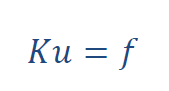
Where K is the global stiffness matrix, u is a vector containing the nodal displacements and f is a vector containing the nodal forces.
However, step by step a non-linear problem needs to be solved. The governing equation for each step then becomes:
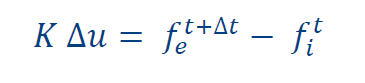
Where Δ𝑢 is a vector containing the nodal displacement increments, 𝑓_𝒆^𝑡+Δ𝑡 is a vector containing the external nodal forces at the end of the increment and 𝑓_𝑖^𝑡 is a vector containing the current internal nodal forces.
To solve this equation, the finite element method starts from an equilibrium state at time 𝑡
when: 𝑓_𝑖^𝑡= 𝑓_𝑒^𝑡 and then a load increment is applied so that: 𝑓_𝑒^𝑡+Δ𝑡= 𝑓_𝑒^𝑡 + Δ𝑓_𝑒 . The method at the end is going to calculate Δ𝑢= (𝑓_𝑒^𝑡+Δ𝑡− 𝑓_𝑖^𝑡) 𝐾^0−1. In order to solve the calculation, the finite element method uses an iterative procedure. At the end of each iteration it calculates the residual force.
If this out-of-balance force is small enough, the equilibrium is reached and the step is ended, otherwise it continues with another iteration. This process will continue until the residual force is small enough to be considered as ‘converged’: a preset ratio between the actual residual force and the initial residual force (norm) at the first iteration.
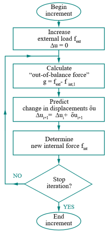
Figure 212 Iteration Process_Diana FEA 10.3.
At the end of this brief explanation about how the finite element method works it is possible to see how the “convergence” is connected to the value of the residual force or residual displacement if also a criterium about the displacement is set in the analysis. This means that “no convergence” is not strictly correlated to the fact that the results are not correct. Non-convergence means that the software has trouble to find the solution and, as a consequence, the engineer has to analyze what is happening around the step in which a convergence has not been found. This is done in order to see if there are issues in the model or not. Can perfectly be that the software has troubles finding an acceptable residual force but that the results are fine.
Note that the convergence is relative to the initial unbalance between external and internal forces.
Usually in the NLPO calculation two convergence criteria are set that need to be satisfied:
Force with a tolerance of 0.01
Displacement with a tolerance of 0.01
If the model is not converging for a value that is close to the limit set for the norm it is still acceptable. If the value of non-convergence is higher, the model should be checked carefully.
Different are the scenario that can happen during a calculation:
At certain step in the model the software cannot find convergence and the message “No convergence” appears in the .OUT file, but after this step it finds again the convergence;
After a certain step the software is not able to find the convergence anymore until the end of the analysis.
In both the case the engineer should investigate the model. In case 1) the step before and immediately after the no convergence should be investigated, in case 2) the behavior of the structure around the moment of no convergence should be investigated.
The parameters that the engineer should check are:
Residual Force: this output can give an indication of the internal forces and show in which point of the structure there are troubles to find equilibrium
Displacement: are the displacement as expected? Or is there a part of the building that is moving in a strange way? (for example: if the analysis is pushing the walls in +X and a wall is moving in -X)
Crack Pattern: The locations of the cracks and the corresponding value can also give an indication about the behavior of the structure.
If, after these checks, the results seem reliable it means that most probably the model is correct; simply the software has trouble to find the solution. In order to validate the model, and continue with the rest of the workflow, a meeting with the knowledge team is required for a last check of the model.
Divergence
The case of “divergence” is different from “no convergence”. Divergence can be correlated to numerical issues (for example in the material settings) or to a structural failure of the building. In this case, it is a good option to try to change the method in the “iterative method” function of DIANA: for example change from Secant (Quasi-Newton) to Netwon-Rapson. If, after this try, the divergence still occurs, it is good to plan a meeting with the knowledge ** **team in order to analyze the model.
More information about this topic can be found in the presentation “Interpretation of Non-Linear Analyses” dated 09 October 2019. Here is the LINK
Step A14: Non-linear flexbase push-over analysis (Optional)
Note
Text to be updated, current developments for NLPO are on hold.
As mentioned in other sections, for NLPO analyses the strengthening measures are not modelled in DIANA. However, for the geo output a non-linear analysis including the weight of the measures needs to be performed.
The nonlinear analysis after adding the weight of strengthening measures is A14a for flexbase analysis and A13a for fixed analysis. The measures are taken into account adding the corresponding additional load directly in the script. After doing it, a non-linear analysis is performed and the forces on the foundation are sent to the geotechnical advisor of the object in a single json-file.
The resulting increment of the base shear forces due to the application of strengthening measures may have consequences at the foundation level, causing the necessity to apply additional strengthening measures at the foundation level. This must be discarded after an additional check. In the NLPO procedure, the foundation or the terrain are not to be considered as elements that may be allowed to fail (so control the maximum shear capacity of the building system)
Further instructions regarding the geo-output will be provided in the next version of the protocol.