How to use the NLPO result template
The template_resultscript_NLPO is used as the template for the result handling of NLPO. This includes two sections:
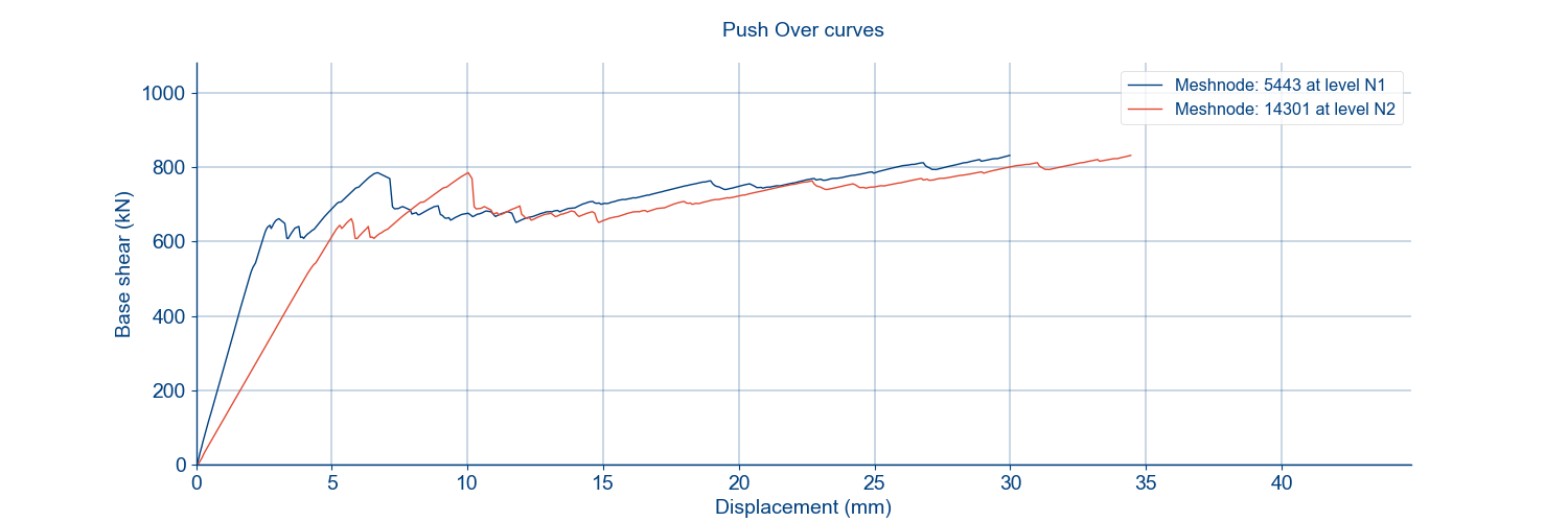
Generation of the plots for pushover curve, bilinearized curve and obtaining the performance point
Generation of the result pictures (This includes the pictures for both the MRS (A5) and NLPO (A11) analysis)
Please install the packages Scipy and Matplotlib in DIANA python before proceeding
Prepare the folder with the result files
Within the A11 analysis folder, make sure to have the folders with following names for the direction - X_pos, X_neg,Y_pos,Y_neg. Within this, choose the dominant load case as either ‘uniform’ or ‘modal’.
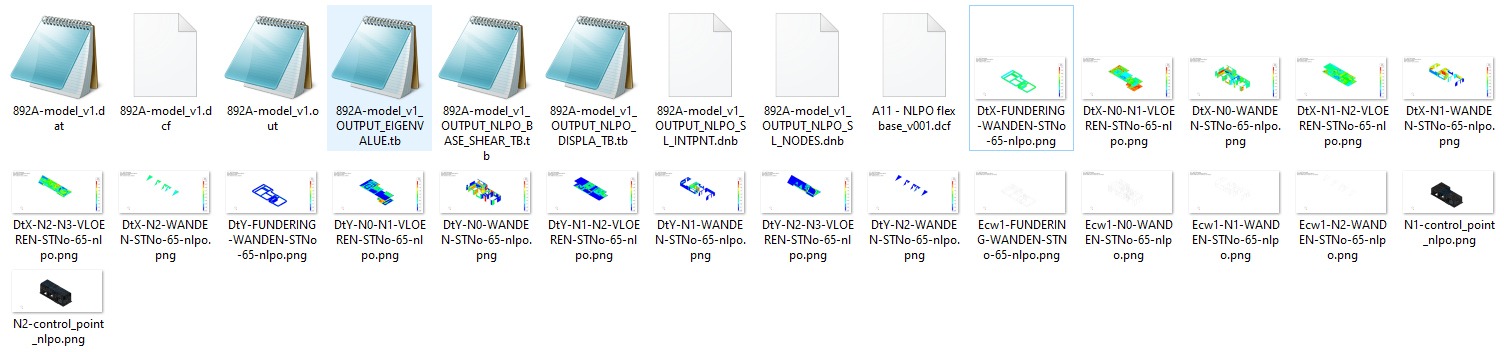
The following result files are needed to obtain the plots and result pictures of the NLPO analysis (A11):
- XXXX_vX.dat (Specific to the NLPO model)
- XXXX_vX.json
- XXXX_vX_OUTPUT_EIGENVALUE.tb
- XXXX_vX_OUTPUT_NLPO_DISPLA_TB.tb
- XXXX_vX_OUTPUT_NLPO_SL_NODES.dnb
The following result files are needed to obtaining the result pictures from the MRS analysis (A5) as part of the NLPO process:
- XXXX_vX.dat (Same as the NLPO model)
- XXXX_vX_OUTPUT_MRS.dnb
The same .json, which is used for NLPO result pictures is also used for generating the MRS result pictures right now.
Make sure the naming is correct!
Section 1 - Generation of the plots for capacity spectrum, pushover curve, bilinearised curve and obtaining the performance point
Step 1 - Read the data
Make sure the names and direction are consistent:
>>> project = viia_create_project(project_name='934A')
>>> workfolder_location = Path("C:\\Users\XXXXXX\Desktop\\test_1")
>>> direction = 'Y' # For the pushover curves
>>> dominant_direction = 'Y_neg' # For generating the result pictures
Then, read the displacement and base shear as dictionary
>>> # The curve for raw data is plotted, check the original curve to determine the cut off step, update the traction accordingly
>>> disp_dict, base_shear_dict, po_curves = viia_read_pushover_curve_data(project=project,
                                                                      work_folder=workfolder_location,
                                                                      direction=direction,
                                                                      traction=False)
Step 2 - Cut off steps
After Step 1, the original pushover curves are plotted in the working folder, discuss with the lead engineer to determine a reasonable cut-off step if necessary. The criteria can be either displacement or base shear.
>>> # Cut it to the step for the first floor where displacement = 30 mm
>>> cut_off_step = po_curves[0].find_cut_off_step(displacement_cut_off=30)
>>> # Cut it to the step for all curves
>>> for curve in po_curves:
>>>     curve.cut_off_step = cut_off_step
Step 3 - Convert into SDOF system
Convert the MDOF into equivalent SDOF system, please check the corresponding properties of the SDOF system.
>>> # Check po.system.eff_mass or any other from ('eff_height', 'gamma', 'po_curves', 'v_star_base', 'u_star_roof', 'roof')
>>> po_system = viia_convert_to_sdof_po_system(project=project,
>>>                                            po_curves=po_curves)
>>> print(po_system.eff_height)
>>> print(po_system.gamma)
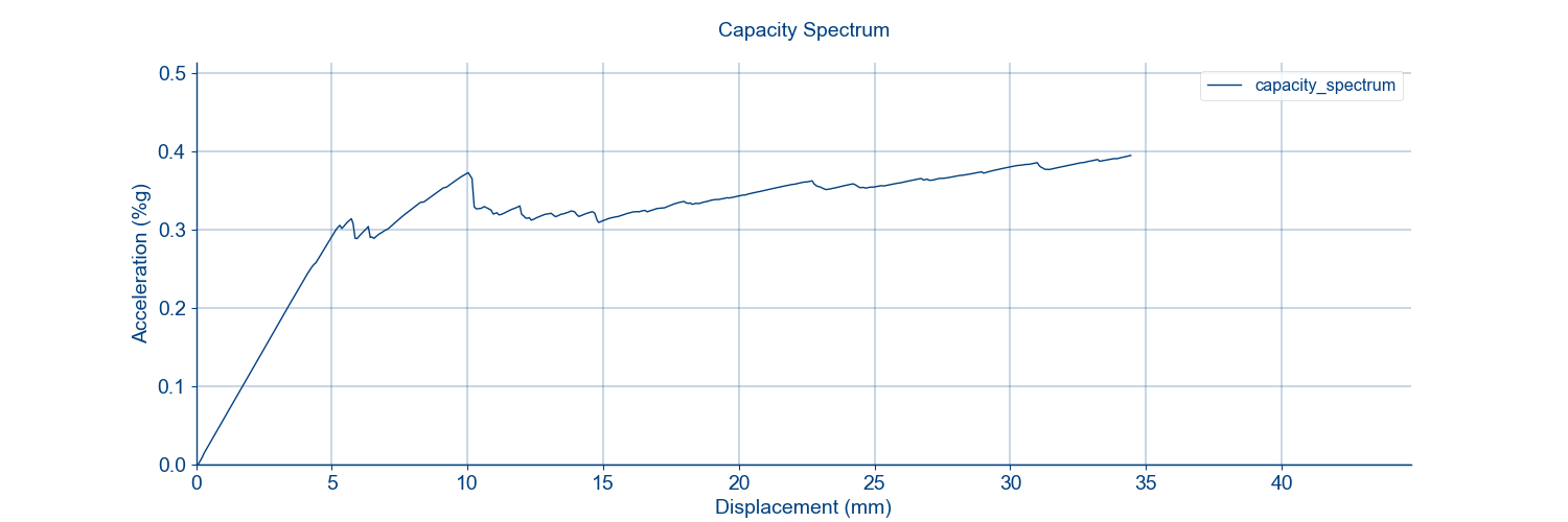
Construct the capacity spectrum if all the above mentioned factor seems correct.
>>> capacity_spectrum = PushoverCurve(project=project,
>>>                                   displacement=po_system.u_star_roof,
>>>                                   base_shear=po_system.v_star_base,
>>>                                   eff_mass=po_system.eff_mass,
>>>                                   direction=direction,
>>>                                   meshnode='system')
Note
Make sure it is bound to the cut off step
>>> capacity_spectrum.cut_off_step = cut_off_step
Then, we should be able to get the capacity spectrum figure in the working folder, check it before proceeding.
>>> PushoverCurve.plot_curve(project, curve_type='CS', input_curve=capacity_spectrum)
The drift limit of the system (ductile in this case) can be checked as well.
>>> drift_limit = viia_get_drift_limit(project=project, po_system=po_system)['dc']
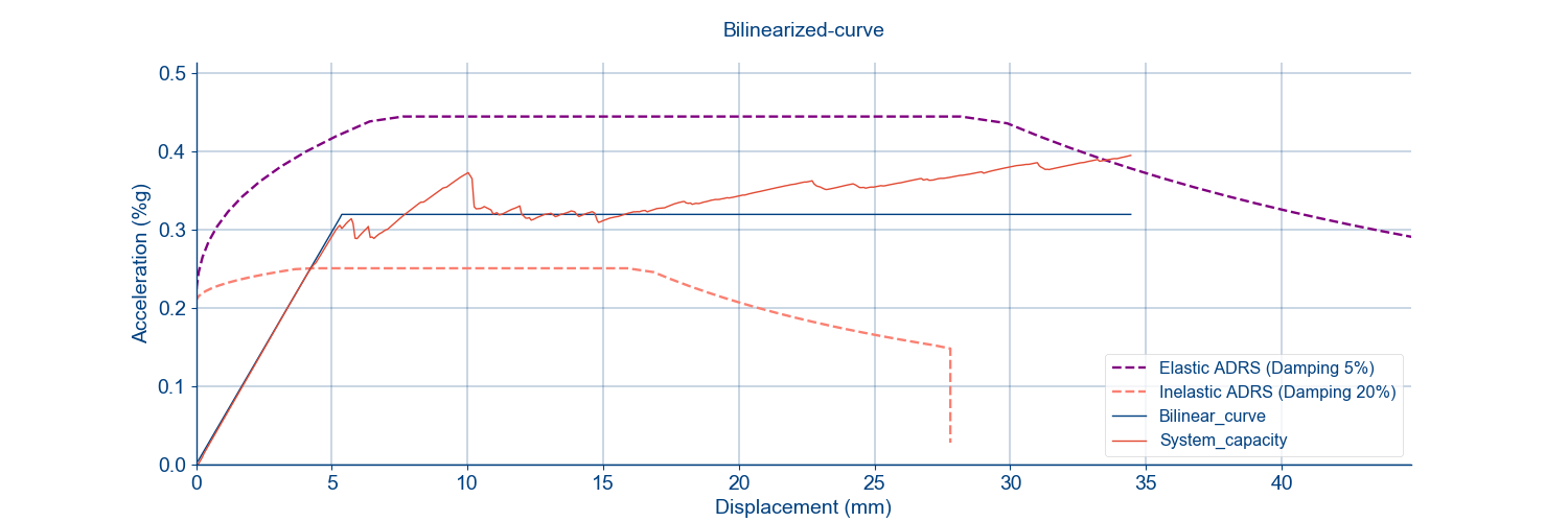
Step 4 - Plot the bi-linear curve
The billinear curve can be plotted after checking the capacity spectrum, the code snippet below will plot the bilinear curve and collect the parameters in the bi_params dictionary. Again, check the parameters if there are numerical issues.
>>> bi_data, bi_params = capacity_spectrum.bilinearise(drift_limit=drift_limit, output_params=True, plot=True)
>>>  print(bi_params) {'K_init': 555491.843796342,
>>>                    'plateau': 0.5173681331215096,
>>>                    'u_capsys': 5.226687447030751, ...
Afterwards, the system ductility and system damping is calculated to initiate the calculation of performance point.
>>> mu_sys = viia_get_sys_ductility_factor(bi_params)
>>> sys_params = viia_get_damping_ratio_correction_factor(mu_sys, failure='dc')
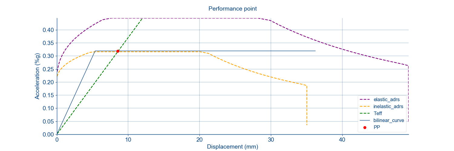
Step 5 - Plot the performance point
If all goes well in Step 4, we should be able to initiate the performance point calculation process, the parameters of the first iteration is collected in the init_cache, which is checked if numerical instability occurs during the calculation process.
>>> # Performance point
>>> init_cache = viia_initialise_performance_point(project, bi_params)
>>> # User should check init_cache if the PP is not found
>>> output_cache = viia_get_performance_point(project, bi_params=bi_params, init_cache=init_cache, error=0.7)
Congrats! You should be able to see the performance point figure after this step, the capacity spectrum is also bound to the performance point step by:
>>> # Find the step corresponding to the performance point displacement
>>> pp_step = capacity_spectrum.find_cut_off_step(displacement_cut_off=output_cache['s_int'])
>>> # The expected performance
>>> capacity_spectrum.cut_off_step = pp_step
Section 2 - Generation of the Result pictures
Warning
This procedure has been updated and is currently not available for NLPO.
After obtaining the performance point in Step 5, this is used as the input for generating the result pictures for the NLPO result pictures. Following this the result pictures from the MRS analysis are generated
>>> # Creation of the NLPO result pictures
>>> project.performance_point = pp_step
>>> project.haskoningDIANA.model_created = True
>>> project.viia_result_pictures(analysis_nr='A11', dominant_direction=dominant_direction)
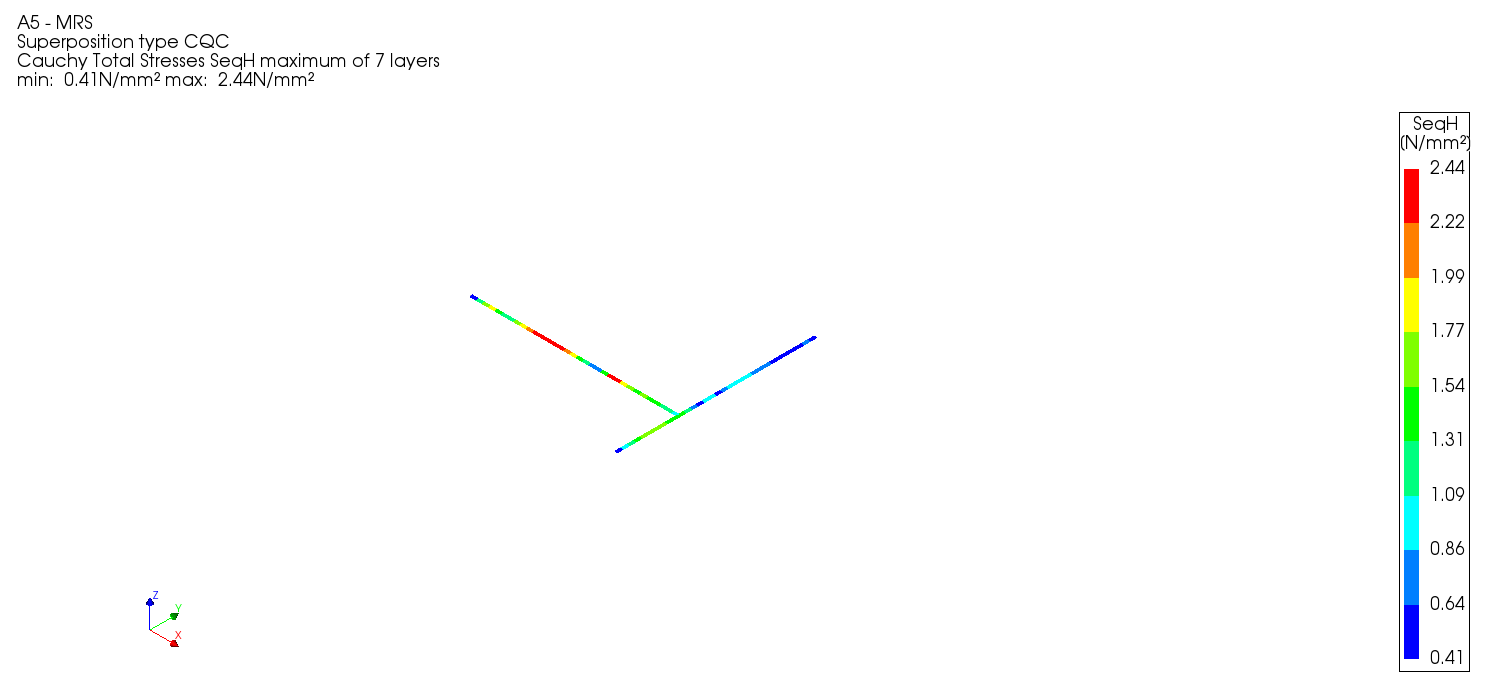
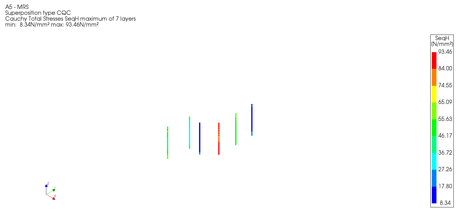
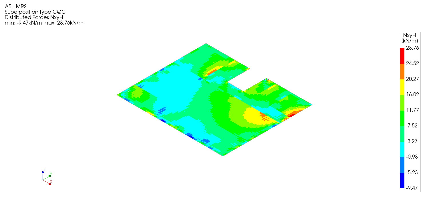
>>> project.viia_result_pictures(analysis_nr='A5', dominant_direction=dominant_direction)
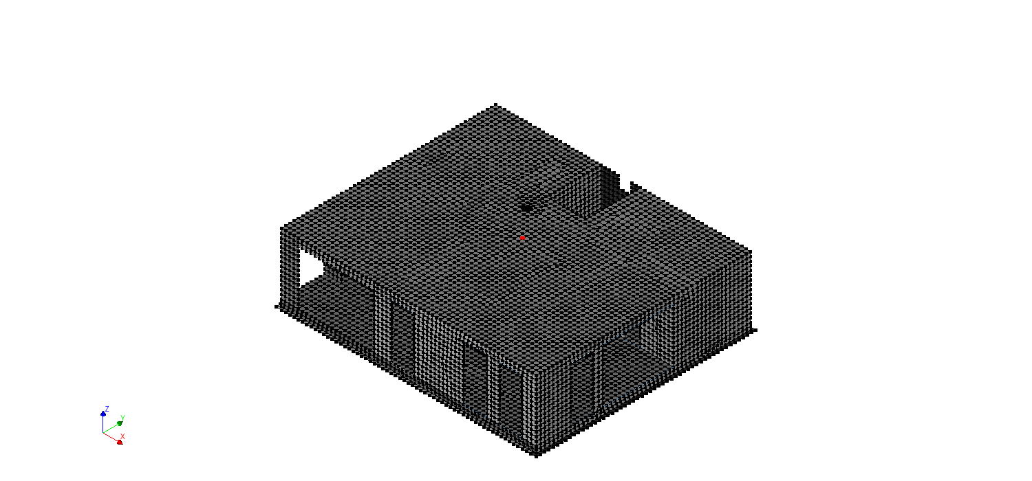
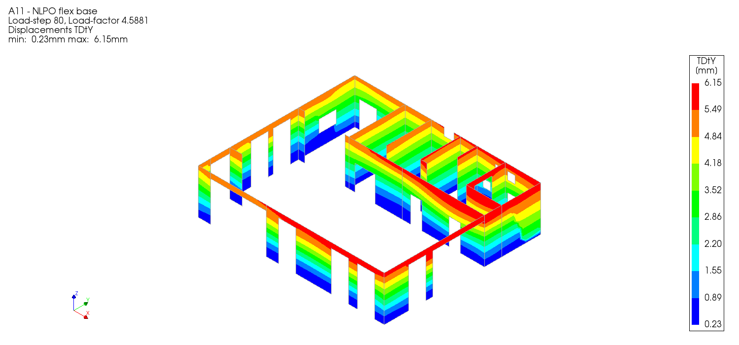
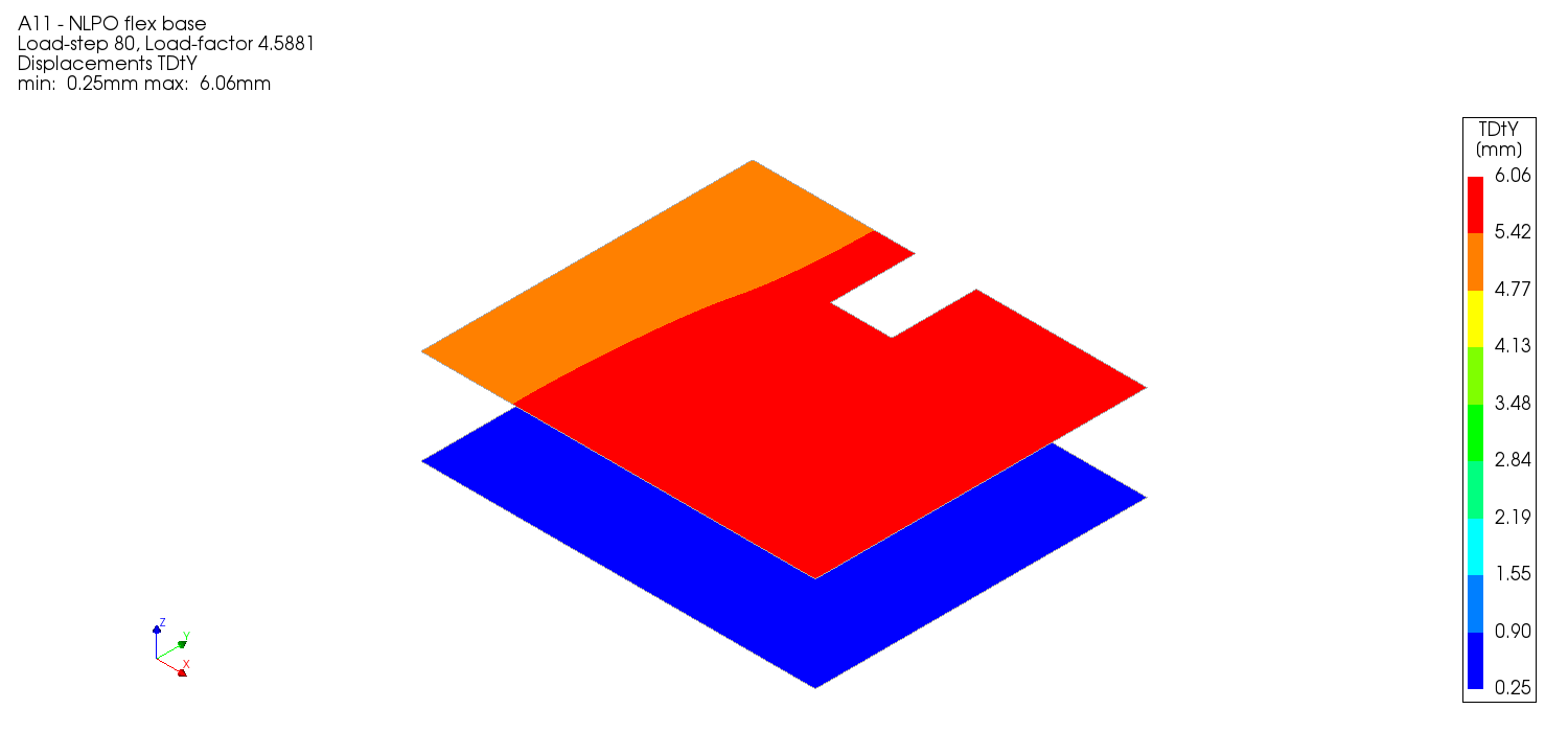
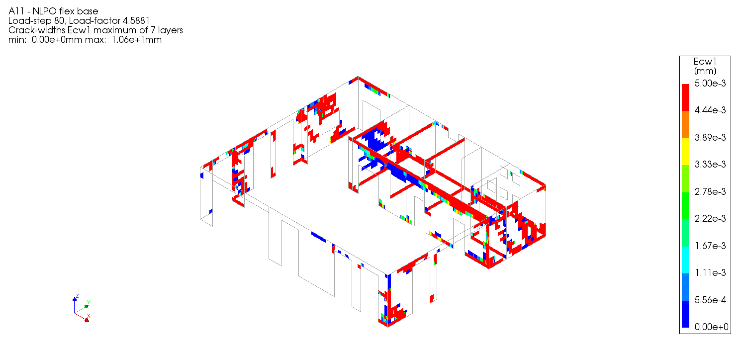
You should obtain all the pictures in the A11 analysis folder. An example is shown in the following image.
The following pictures should be generated. Example pictures are added at performance point of 80.
A11 analysis folder:
- Control point per storey
- Wall displacements (TDtx and TDty) per storey at performance point
- Inter-storey drifts (TDtx and TDty) per storey at performance point
- Crack-widths (Ecw1) per storey at performance point
- Floors and roofs based on material and storey (NxyH)
- Beams and Columns based on material and storey (SeqH (maximum of 7 layers))