How to modify analysis in abaqus
While running analysis in ABAQUS, some changes needs to be made in the model. Be it in defining the analysis, changing material properties, changing interface properties or some changes in the building that cannot be done using the VIIApackage. This section explains the changes that needs to be made while running the A10/A13 and A12/A15 analysis in ABAQUS.
Changes in Non-Linear Static Analysis A10/A13
This section involves the changes required in ABAQUS model while running the A10/A13 analysis.
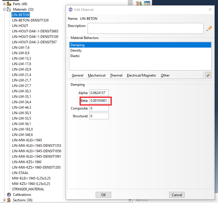
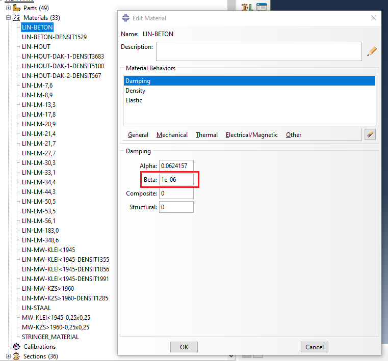
Change the beta value of all the materials (except the line mass and the non-linear masonry model) to 1e-06. This helps in keeping the mass scaling factor (EMSF) to be within 1e-02
Add the rotational stiffness of 1000 N/m, in all three direction, to all the point interface properties.The rotational stiffness should also be added to the Hinge material properties.
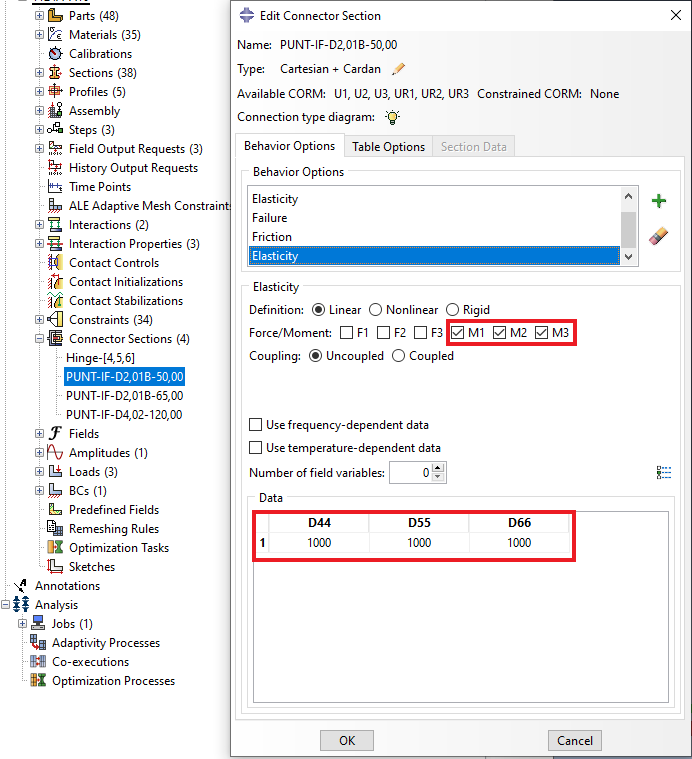
Figure 216 Addition of rotational stiffness to all the point interface properties.
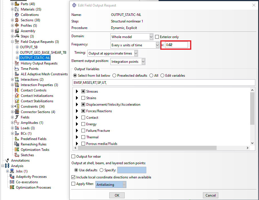
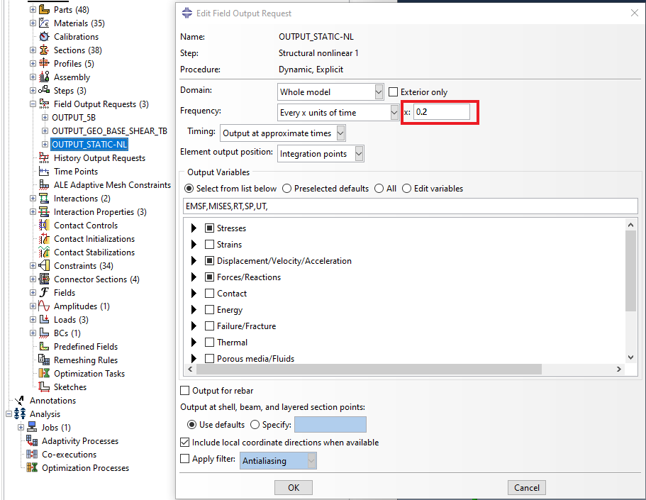
Change the stepsize from 0.02 to 0.2 for all the output blocks under the ‘Field Output Requests’.
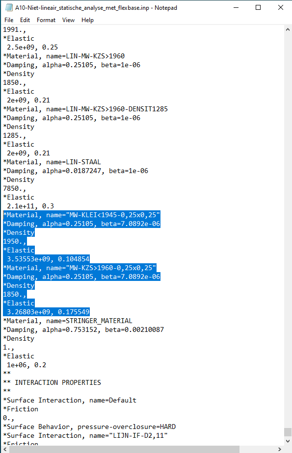
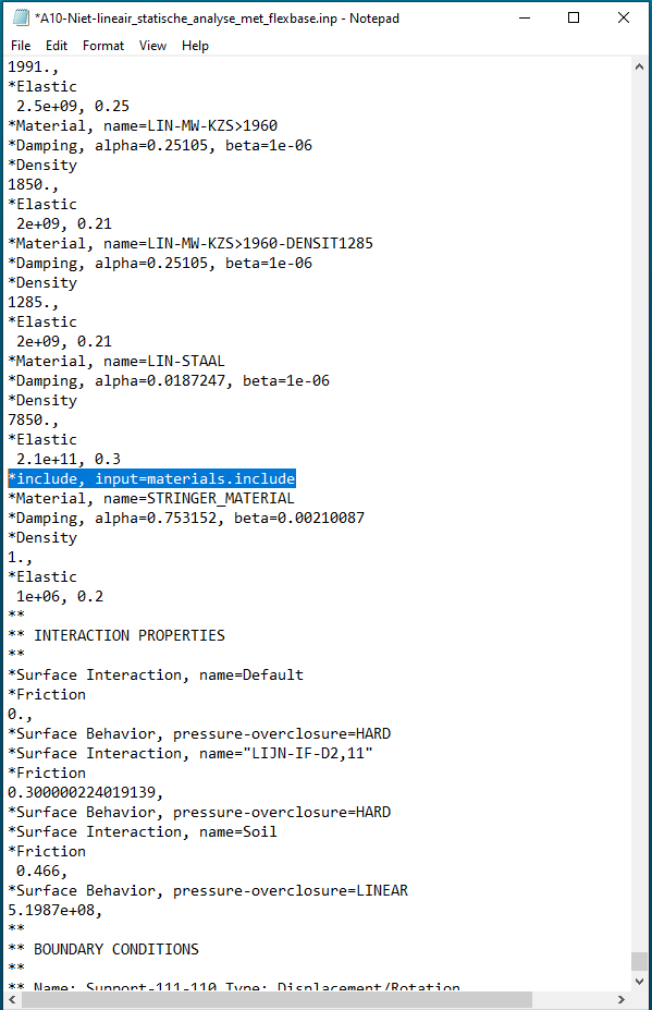
In the input file (inp-file), remove the non-linear masonry material properties and add the code *include, input=materials.include
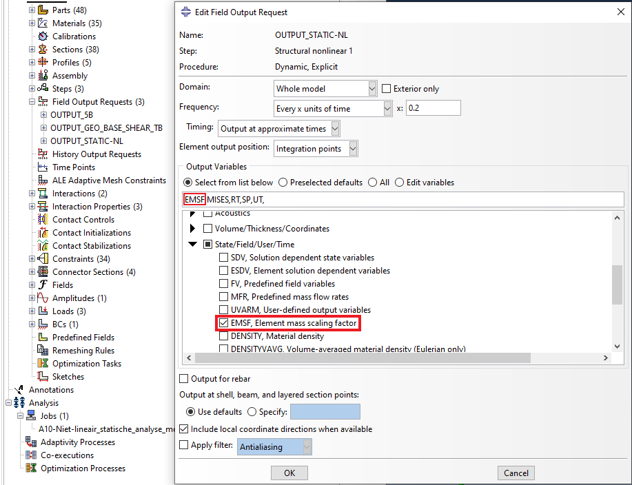
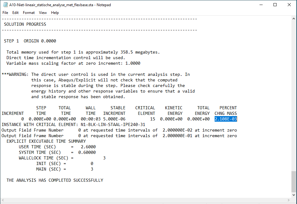
The EMSF value should be checked before running the A10 analysis. This can be referred to :ref: Element_mass_scaling_factor_check. The check can be performed by adding the output (EMSF) to the output block named “OUTPUT_STATIC-NL” as shown in Figure 8 and perform the data check on the object. Once the data check is performed, status file (.sta) is generated in the analysis folder. Check the file for percent changing mass and make sure it is less than 1e-02 (factor of 1e-04). If not, change the mesh size of certain parts of the object and check the EMSF value again or change the geometry.
Changes in Non-Linear Time History Analysis (A12/A15)
This section involves the changes that are needed in the ABAQUS model while running A12/A15. The EMSF check, changing beta value, adding rotational stiffness to point interface properties and replacing the non-linear material property lines in the input file remains the same as mentioned for A10/A12 analysis. Additional changes required in the NLTH analysis are shown below
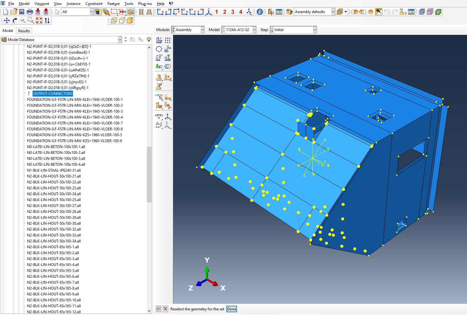
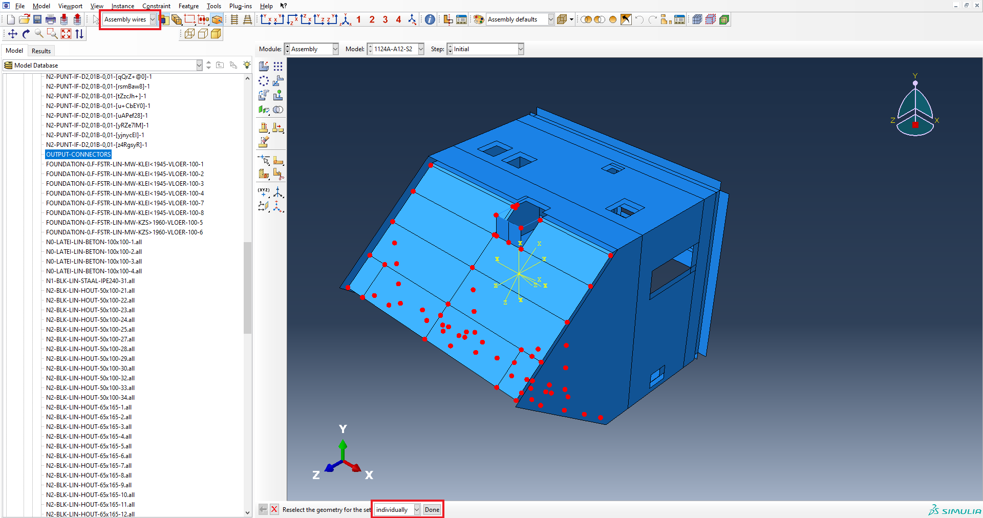
With the VIIApackage, the ‘OUTPUT CONNECTORS’ under sets in the assembly is not selected as shown in Figure 10. This can be done manually by changing the cursor selection from ‘All’ to ‘Assembly Wires’, selecting all the connections in the building and clicking done.
While generating A12 analysis, the time period for ‘Structural Nonlinear 2’ is constant at 12.5 seconds. For some signal, this might not be correct as the time signal can be greater than or less than 12.5 seconds. The total time for a signal can be checked in the ‘Amplitude’ section of the model tree. If there is a discrepancy observed in the time period, then change the value in ‘Strutural Nonlinear 2’ step.
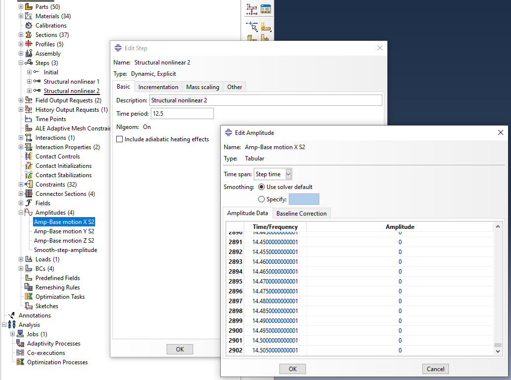
Discrepancy in time period value. Time period in Structural Nonlinear 2 is 12.5 seconds whereas the signal continues to 14.5 seconds. In this case, change the time period value in ‘Structural Nonlinear 2’ to 14.5 seconds
The stepsize for the output blocks needs some changing. The step size for ‘Structural Nonlinear 1’ under the output block ‘OUTPUT_NONLINEAR’ and ‘OUTPUT_NONLINEAR_CONNECTORS’ in the ‘Field Output Requests’ needs to be changed from 0.02 to 0.2. The step size for ‘Structural Nonlinear 1’ under the output block ‘OUTPUT_NONLINEAR’ and ‘OUTPUT_NONLINEAR_CONNECTORS’ in the ‘Field Output Requests’ needs to be changed from 0.2 to 0.02. Finally, the step size for the output block ‘OUTPUT_NONLINEAR_HISTORY’ in the ‘History Output Requests’ needs to be changed from 1E-100 to 0.002.
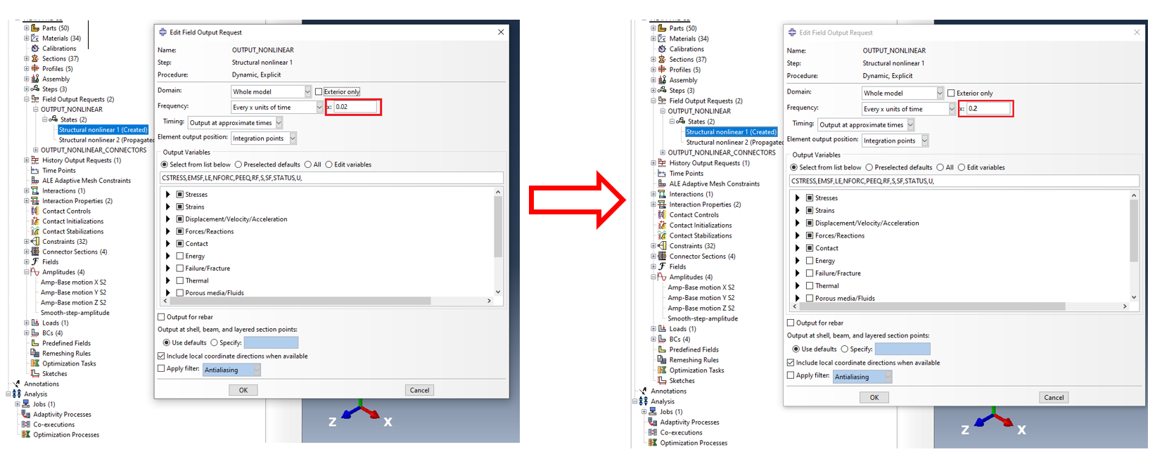
Figure 225 Change in step size for Structural Nonlinear 1 from 0.02 to 0.2. This should be done for both the output blocks under ‘Field Output Request’.
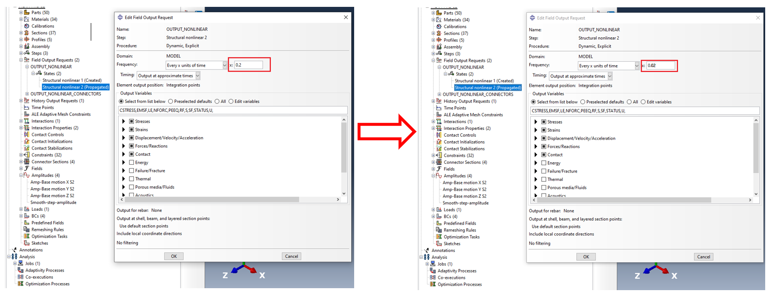
Figure 226 Change in step size for Structural Nonlinear 2 from 0.2 to 0.02. This should be done for both the output blocks under ‘Field Output Request’.
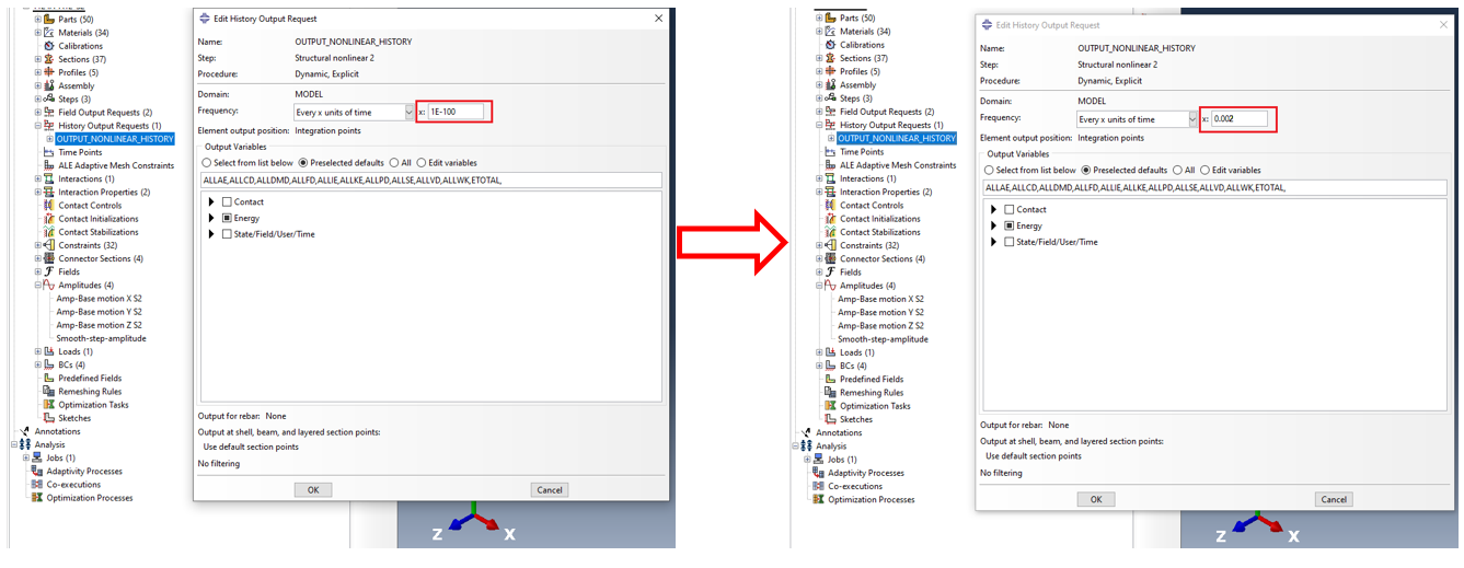
Figure 227 Change in step size for history output block from 1E-100 to 0.002.