How to select the critical pushover curves

A procedure how to determine the most critical capacity pushover “PO” curve for each of the main building directions, referred normally as “x” and “y”, is presented in this document. The process is explained for both the simple NLPO analysis, where the mass can be assumed to act at the rigid floor (single-system) and the subsystem NLPO, where the building mass is divided into separate individual SDOF according to the distribution of the seismic resistant elements (usually one seismic resistant subsystem for each architectural axis with presence of structural components).

As aid to determine the criticality of a PO curve, the reference seismic demand spectrum, at the location of the building, is plotted in the acceleration-displacement spectral response graph (ADRS) for hysteretic damping values of 5% and 20%.

Abbreviations and symbols

The following are symbols, notations and abbreviations used throughout this document in other to determine the most critical PO curve to be used in the NLPO analysis method:

• ADRS Acceleration-Displacement Response Spectra

• CS Capacity Spectrum

• MDOF Multi-degree of freedom

• NC Near collapse

• SDOF Single degree of freedom

• g acceleration of gravity (9.8 m/s2)

• h_eff Effective height of the equivalent SDOF system

• m_eff Effective mass of the equivalent SDOF system [kg]

• m_i Seismic mass at the story at level i [kgm] (definition in UPR and Protocol)

• S_a Spectral acceleration

• S_d Spectral displacement

• S_e(T) Elastic acceleration response spectrum for period T

• S_De(T) Elastic displacement response spectrum for period T

• S_e,n(T) Inelastic acceleration response spectrum for period T

• S_e,n(T) Inelastic displacement response spectrum for period T

• S_d,ξsys (T_eff) Target displacement (demand) at the effective period T_eff

• u_dak top displacement (at control point) of the MDOF system

• u*_dak top displacement (at control point) of the SDOF system

• V_fund Base shear force of the MDOF system

• V*_fund Base shear force of the SDOF system

• Γ Transformation factor

• η_sys System damping correction factor

• η_ξ spectral reduction factor

• Θ_R,NC,f Drift limit for rocking (flexural) for URM piers/walls in the NC-state

• Θ_R,NC,v Drift limit for rocking (shear) for URM piers/walls in the NC-state

• μ_sys Global structural ductility of the system

• ξ_sys Equivalent viscous damping ratio

Obtaining and plotting the seismic demand curve

Only the PO curves themselves may not provide enough information to assess what curves are critical or, in case of subsystem NLPO curves, if not only one but various subsystems may face difficulties to sustain the expected seismic load. The steps to find the elastic and inelastic seismic demand curves in ADRS format is described as follows:

Step 1: Get the seismic input

Load the webtool page: https://seismischekrachten.nen.nl/map.php, indicate the address of the object of interest and choose the other parameters (Time period (= T1), Return period (usually = 2475 years) and Direction (= horizontal)). Refer to the starting points document to select the proper parameters to use in the webtool in case of doubt. Then the seismic data of this address (a graph and parameters) will be presented. Pick up the following parameters:

• a_g S [g] peak ground acceleration at the surface level (incl. soil factor)

• p [-] seismic response amplification factor

• T_B [s] lower limit of the period in the constant spectral acceleration branch (lower corner frequency)

• T_C [s] upper limit of the period in the constant spectral acceleration branch (higher corner frequency)

• T_D [s] value defining the start of the constant displacement response spectrum

Step 2: Plot the elastic seismic demand in the ADRS space

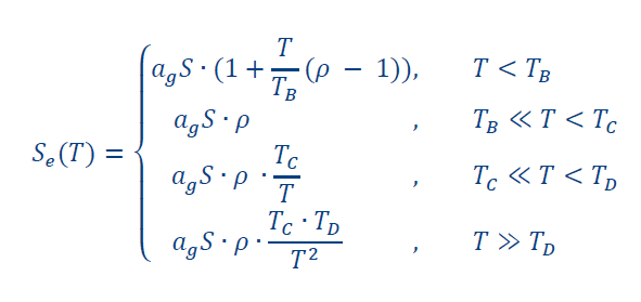
1. Elastic acceleration response spectrum: S_e (T)

The following equations are used to formulate the elastic acceleration response spectrum according to the values determined in step 1:

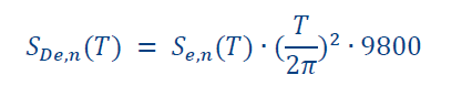
2. Elastic displacement response spectrum transformation: S_De (T)

The response in terms of the spectral displacement spectrum can be obtained by means of the following transformation from the acceleration response spectrum:

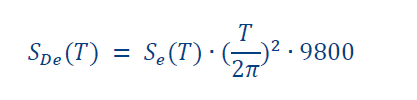
*Note: the value 9800 here is a unit conversion factor for gravity acceleration “g” from [m/s2] to [mm/s2] (spectral displacements in mm)

3. Plot the elastic demand curve in the ADRS

The elastic ADRS demand curve is generated by plotting the S_e (T) versus S_De (T). An example of this is shown in Figure A1.

Step 3: Plot the inelastic seismic demand in the ADRS space

During earthquakes, energy is released due to processes such as the formation of plastic hinges in the structures (structural response in the non-linear range) and soil structure interaction, “SSI”. The effects of these processes reflect in a reduction of the magnitude of the response; so, the amplitude of the response is damped. Structures can damp forces in the elastic range according to their inherent structural damping (usually considered as 5%). In nonlinear analyzes, the amplitude of the response is further damped by the inelastic behavior of the structure (usually reflected well by the ductility factor).

For unreinforced masonry structures, “URM”, a reference value of inelastic damping of about 20% may be used as maximum for low-rise story building (Table G.3 in NPR:9998-2018). As an initial estimation of what may be the most critical PO curve, this reference value can be used as a decision-making parameter and to have already an idea if the structure will comply or not with the NPR:9998-2018 regulations. The inelastic ADRS demand curve can be obtained through multiplying the elastic ADRS with a spectral reduction factor η_ξ, which can be calculated using the following equation:

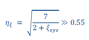
where ξ_sys [%] is the equivalent viscous damping (a value of 20 can be used here). *Note: the equivalent viscous damping is to be calculated later based on the achieved structural ductility and the observed inelastic mechanism. Detailed explanations on this can be found in NPR 9998-2018, G.7.4.

After calculating the spectral reduction factor η_ξ, the inelastic acceleration response spectrum can be obtained through:

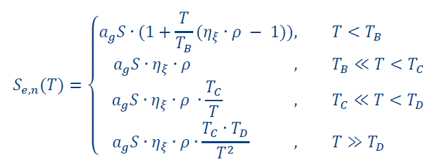
Similarly, the inelastic displacement response spectrum is calculated as:

The inelastic ADRS demand curve is generated by plotting the S_e,n (T) versus S_De,n (T). See an example plot in Figure A1.

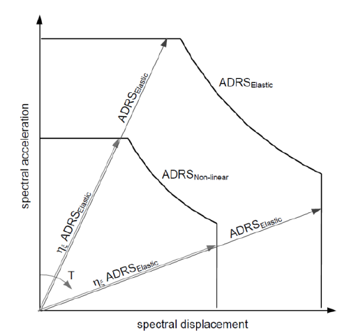
Figure - A1: elastic/inelastic ADRS demand curve (fig. G.7 NPR)

Obtaining the capacity spectrum ‘CS’ from pushover curves

Based on the displacements at the control nodes (observe differences in the location of the control point in the stating points and the NLPO protocol documents) and the base shear force outputs from DIANA, the PO-curves correspondent to the MDOF system can be plotted.

By the conversion of the MDOF into a SDOF and the normalization of the base shear to the effective mass, the capacity spectrum “CS” is obtained (review the staring points document and the protocol document). The CS describes the global expected behavior of the structure and can be directly contrasted with the seismic demand after plotting the CS in the ADRS. This process varies according to the type of NLPO analysis performed, single-system NLPO (whole structure) or subsystem NLPO. Variations are commented in this chapter.

It’s important to mention at this moment, that even if they are not included in DIANA model, the outer walls and other non-structural masses, such as chimneys, should be considered for the seismic mass calculation with is used in the calculation of the spectral capacity. To perform the conversion from a MDOF to a SDOF system, the following steps can be followed:

Step 1: Compute the effective mass of the equivalent SDOF system: meff

The equation to calculate the effective mass is as follows:

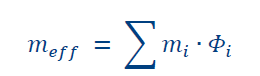
where m_i is the seismic mass at story i, and Φ is the unitary displacement at each level. For the nodal load pattern, Φ can be initially estimated from the DIANA output by inspecting the eigen-shape of interest according to the eigenvalue analysis. This pattern should be later verified by the observed Φ elastic values at each level of the MDOF system (can be estimated at 60% of the maximum lateral capacity). Differences related to the each NLPO variations are the following:

Seismic mass for single-system NLPO analysis:

• The mass at 1st storey: m1 [kg] is the sum of the weight of following elements:

  ▪ Top half of the walls on the ground floor ▪ The first floor ▪ Bottom half of the walls on the 1st floor

• The mass at i-th storey: mi [kg] is the sum of the weight of following elements:

  ▪ Top half of the walls on the (i-1)th floor ▪ The i-th floor ▪ Bottom half of the walls on the i-th floor

• The mass at the top storey*: mn [kg] is the sum of the weight of following elements:

  ▪ Top half of the walls on the (n-1)th floor ▪ The n-th floor ▪ The roof

Note

Structures with big roofs usually present 2 attic level (lower and upper attics as in Figure A 2). This situation is proposed to be modeled for URM structures in two ways according to what it can be observed in the figure. There, in Figure A 2.a, an extra mass located at the upper attic level is assumed if the internal walls located at the lower attic are URM and load bearing. For this case, an internal continuous was observed in “x” direction and is linked to the lower attic gable external walls in “y” direction configurating the lateral structural resistant system in both directions. Structural internal walls are not common in lower or upper attics floors and mostly the structure in the attics consist mainly of steel or wooden trusses/frames. For this condition, the URM gables in Figure A2 are to be secured against the out of plane failure mode and the MDOF formulation follows the one of Figure A2.b, with all the mass concentrated at the floor of the lower attic level.

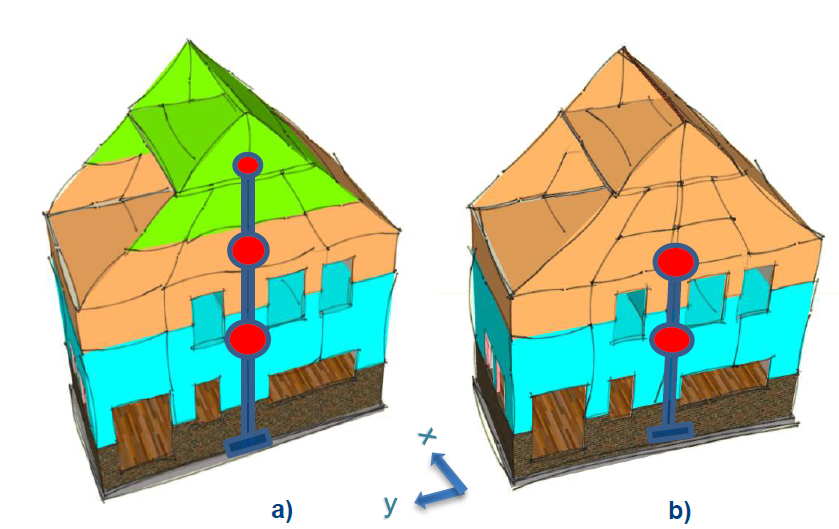
Figure - A2: Formulation of the MDOF system for two levels attic (note that the roof on one side of the building is hidden). This MDOF is valid if a rigid diaphragm condition is observed in at least the 1st level and the lower attic floors. If only the 1st floor is concrete the suitability NLPO method to analyze the structure must be addressed.

Seismic mass for subsystem NLPO analysis:

Here, the seismic mass to be used to estimate as the effective mass should be calculated per subsystem. This condition implies that different form the single-system NLPO the mass at each story should be divided per seismic structural resistant line. The number analyzed subsystem depends on the layout of the walls, on the floor types and span directions. Overall, to observe the load flow from the roof to the foundation is important the determine the seismic mass of each subsystem and every object present its particular conditions; therefore, engineering judgement is required to estimate the allocations of masses.

Regarding the load flow from timber floors, an example of how to calculate the effective mass per subsystem for two different floor support condition is given in Figure A3.

In Figure A 3, the subsystems in “x” and “y” directions are numbered as X1 to X5 and Y1 to Y5 respectively. Now, let’s look to what will be the accounted seismic mass from timber floors for subsystems in “x”, with emphasis in the subsystem line X5:

- Case 1 (Figure A 3.a): all floors are supported on walls in the “x” direction. The load distribution from the floors in terms of the tributary area is simple since is in all cases half of the spanning floor length. Apart from the mass from the floors, the walls mass in the perpendicular “y” direction are also to be added. This can be observed in Figure A 3 for the X5 axis (red walls in “y” direction).

- Case 2 (Figure A 3.b): the spanning direction of some floors varies creating a situation where the mass carried in the “x” direction from the floors is also transferred by the walls in the “y” direction producing a more complex load distribution situation. Here, it should be noticed that the condition marked by the doted red circle can be simplified to the one of the purple slashed line circle.

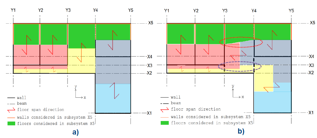
Figure -A3: Allocation of timber floor masses according the spanning direction of the floors.

In Figure A 4, the seismic mass distribution for similar buildings to Figure A 2 is done; just, this time they present flexible timber diaphragms, so the subsystem formulation is required. In the figure the sketches a) and b) represent the structure with structural elements in the lower attic and sketches c) and d), the one with no structural walls in the lower attic.

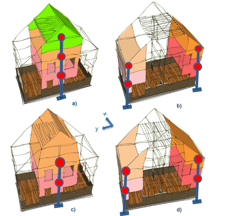
Figure -A 4: Formulation of the MDOF subsystems for a two levels attic (note that the roof on one side of the building is hidden) in the “x” direction with (a & b) and without (c & d) structural walls in the lower attic.

Its usual that URM structures with flexible timber floors in the Groningen area present complex layouts, including structural additions and modifications performed during the life span of the building. In practice, this creates complications to understand clearly the load paths for the seismic mass determination per each of the subsystems formulations. Because of this, it’s recommended to limit to a maximum two stories buildings the subsystem NLPO method (excl. attic). A higher number of stories can be considered for buildings with regular layouts and, in opposition, only one level for buildings with uncertainties (materials, construction details, etc) and irregular layouts.

If the subsystem masses are not to be calculated as commented previously due to extensive work required, an approximate procedure only applicable to a one-story building estimates the seismic mass based one the observation of the reactions at the foundations as follows:

1. Perform the static analysis (only self-weight is applied). Request the vertical reactions at the foundations. Include the mass of the outer wall in cavity walls and other NSE.

2. Determine the effective foundation part for each subsystem (see an example in Figure A 5). The effective foundation part can be simply extracted by considering the foundation under the walls in the analyzed assessment line (X5), and the foundations under half of the walls in the other direction (Y direction) that are connected to the wall in X5.

3. Get the summation of the reaction forces for each foundation subsystem, from which the effective mass of each subsystem can be estimate approximately by dividing this sum of reactions force by g and multiplying by a factor of 0,70 (this factor is conservative and is intended to extract the mass of the foundation and the lower half of the walls from the ground level). If the walls are observed to present lower capacity than expected following this procedure, a detailed calculation of the seismic mass per subsystem is recommended.

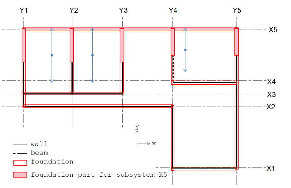
Figure -A 5: Example of the foundations used to calculate the seismic mass acting in the X5 axis.

Step 2: Compute the transformation factor: Γ (same for both NLPO)

The transformation factor “Γ” transforms the base shear forces and displacements of the MDOF system to those of the quivalent SDOF system. Based on the calculated meff and the elastic displacements at each level Φ, the transformation factor Γ can be calculated with:

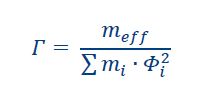
*Note: For URM buildings with a maximum of 2 stories (excl. attic), the transformation factor can be assumed to be 1 (Γ = 1) according to the NPR:9998-2018.

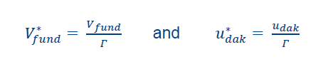
Step 3: Calculate the base shear force and displacement of the SDOF system: V*fund and u*dak (same for both NLPO)

With the Γ factor from step 2, V_fund and displacement at the upper level (u_dak) of the MDOF system (inputs for the PO-curves in Section 2), the base shear force (V*fund) and displacement (u*_dak) of the an equivalent SDOF are attained by dividing both V_fund and u_dak by Γ:

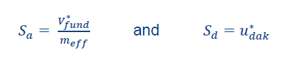
Step 4: Calculating the spectral capacity curve: Sa, Sd (same for both NLPO)

The spectra acceleration Sa and spectra displacement Sd are obtained by:

With the obtained S_a and S_d in step 4, it can be now plotted the spectral capacity curve of the system/subsystem in ADRS format so that it can be directly compared with the seismic demand. For single system NLPO, two capacity curves are plotted for each analysis direction (+X, -X, +Y and -Y directions) corresponding to each load case (minimum two PO load pattern cases, usually the uniform and the modal). For a subsystem NLPO, two capacity curves per subsystem for each one of the four directions is plotted (usually the uniform and the triangular patterns) and the curves from all involved subsystems in the correspondent direction are plotted together (+X, -X, +Y and -Y). An example of the obtained capacity spectrum curves for five subsystems from the uniform load pattern in the +Y direction is shown in Figure A 6.

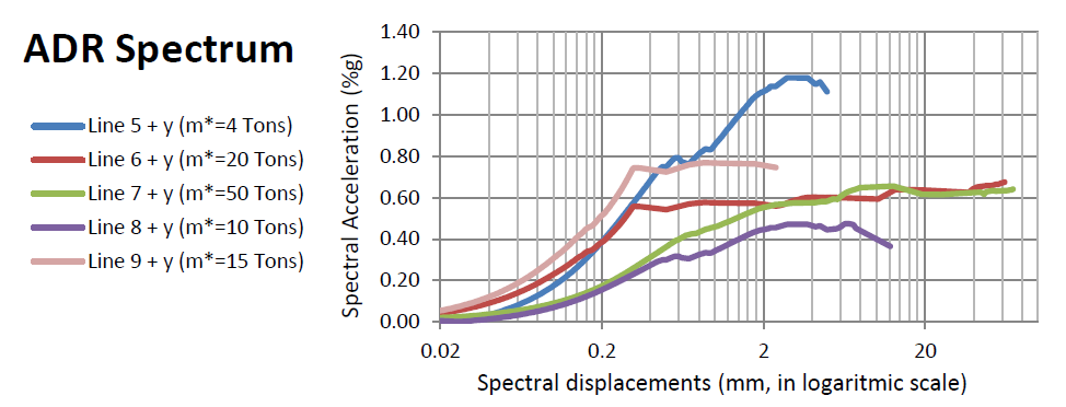
Figure -A 6: Spectral capacity curves in the +Y direction form the uniform load pattern for 5 subsystems (seismic masses per subsystem are in the parenthesis) in a one-story building (seismic mass is equal to the seismic mas in this case)

It can be observed from Figure A 6 that once the PO curve is divided by the meff, the spectral capacities of Line 6 and 7 are similar, even if the original base shear capacity of line 7 is about 2.5 times higher. This comparison makes evident the importance of estimation properly the seismic mass of the building.

Choosing the ‘most critical’ capacity spectrum curve

As required in NPR:9998-2018, for each system/subsystem, a ‘most critical’ capacity curve should be selected for each analyzed direction. Depending on the structure behavior, curves also must be tagged as ‘ductile’ or ‘brittle’. The ‘most critical’ curve can be identified by inspecting the curves, the crack pattern and/or by estimating the failure modes (NPR 2018 G.9). Other aids are to check the sequence of Diana images (or video) close to the start of the non-linear behavior and to observe the convergence iteration data. These are all aspects that support engineering judgement to finally select the capacity spectrum curve governing the analysis for each to the two main resistant directions (“x” and “y”).

For single-system NLPO, at least four curves are two be analyzed in the “x” direction and four in the “y” direction. These four curves can be plotted together with the elastic and the 20% damping inelastic seismic demand as a support to identify the ‘most critical’ capacity curve of the system to be selected for each analysis direction.

For subsystem NLPO, the procedure is the same as for the single system NLPO with the main difference that the amount of analyzes is to be multiplied by the number of subsystems. So, for the five subsystems in the “y” direction, the most critical curve is to be decided after analyzing twenty CS curves (4x5=20) only for that direction.

A strategy to determine the cortical curve is to evaluate all twenty curves in the same graph (may be confusing) or to reduce the number of curves to four by selecting the most critical subsystem per load case as it can be observed in Figure A 7. The latest is preferred as this part of the process is visual and because it allows to observe if more than one of the subsystems may be critical.

To select the dominant/critical curves, additional information is useful to be compared with the capacity spectrums: the elastic and inelastic seismic demand, and maximum allowed drift limits (NPR:9998-2018 G.6.1). The last, is a trim value for the capacity spectral curve and depends of the expected failure mechanism. The seismic demand, on the other hand, is useful not only for the decision making about the most critical situation but also for the following:

• For subsystems with high base shear capacity it allows to observe if the subsystem is compliant in the elastic range to the seismic demand even if their CS curve don’t reach the plastic range. This only applies to the subsystem formulation where all subsystems are pushed at the same time. Because of this last aspect, the amount of loading steps may not had been enough for subsystems with high base shear capacity to yield; but, to observe that they comply in the elastic range is enough to avoid the necessity to conduct again the PO analysis with, for instance, wider loading steps that may bring numerical difficulties to low base shear capacity subsystems (this observation applies only to subsystem NLPO).

• To compare with the seismic inelastic (ξ=20%) and elastic (ξ=5%) demand will already give a good idea if the structure will comply or not with the NPR, even if the curves have not been bi-linearized and the performance point “PP” has not been found. This process will also be able to identify if various subsystems are expected to be not complying with the NPR which is important information later to define in-plane retrofitting measures since these measures are to be employed per subsystem and not necessary to the whole structure.

• To note if the subsystems are expected to perform in the elastic or inelastic range.

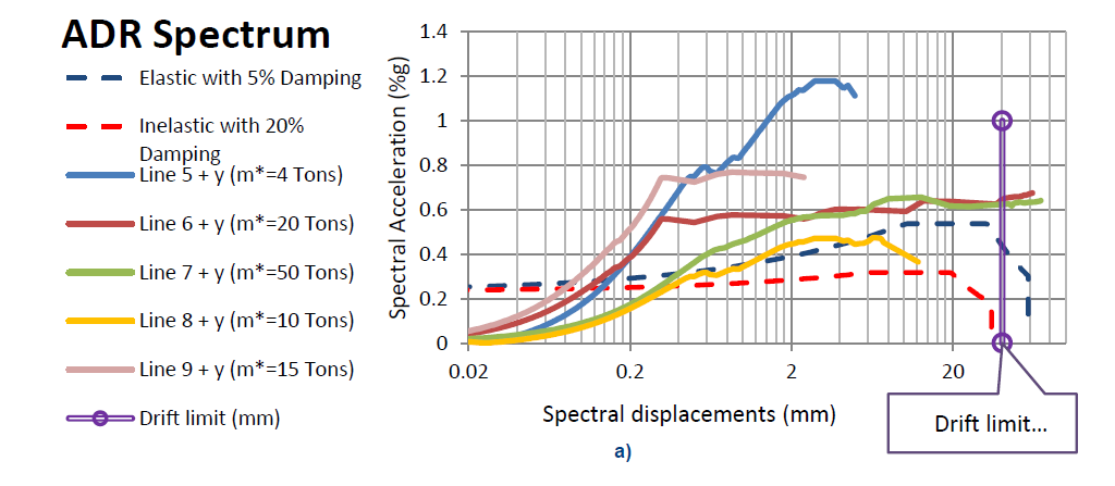
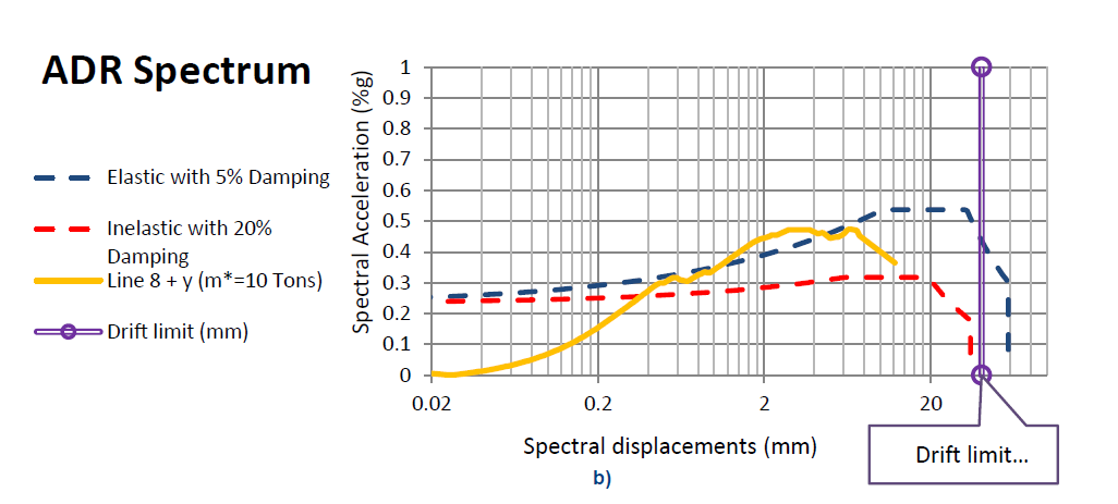
Figure -A7: Selection of the critical spectral capacity curve in the +Y direction form the uniform load pattern for 5 subsystems (seismic masses per subsystem are in the parenthesis) in a one-story building. a) all subsystem plotted together with the seismic demand and drift limit and b), selection of the critical case for +Y and uniform load case.

The selected curve in figure A7b is the one to be bi-linearized according the NPR 9998:2018 NLPO process. The performance point “PP” to that bilinearization is to be obtain as commented in annex B of this document. For the other curves observed in figure A7b, the associated performance point is the one estimate at the intersection of the capacity spectrum curve with the elastic seismic demand. Its possible that more than one curves are considered critical if the resultant bilinear CS curve plateaus are below the inelastic ADRS.